NicheNet example

workflowr

• Summary
• Checks
• Past versions

Last updated: 2020-11-24

Checks: 7 0

Knit directory: interaction-tools/

This reproducible R Markdown analysis was created with workflowr (version 1.6.2). The Checks tab describes the reproducibility checks that were applied when the results were created. The Past versions tab lists the development history.

---

R Markdown file: up-to-date

Great! Since the R Markdown file has been committed to the Git repository, you know the exact version of the code that produced these results.

Environment: empty

Great job! The global environment was empty. Objects defined in the global environment can affect the analysis in your R Markdown file in unknown ways. For reproduciblity it’s best to always run the code in an empty environment.

Seed: set.seed(20191213)

The command set.seed(20191213) was run prior to running the code in the R Markdown file. Setting a seed ensures that any results that rely on randomness, e.g. subsampling or permutations, are reproducible.

Session information: recorded

Great job! Recording the operating system, R version, and package versions is critical for reproducibility.

Cache: none

Nice! There were no cached chunks for this analysis, so you can be confident that you successfully produced the results during this run.

File paths: relative

Great job! Using relative paths to the files within your workflowr project makes it easier to run your code on other machines.

Repository version: 0333fe3

Great! You are using Git for version control. Tracking code development and connecting the code version to the results is critical for reproducibility.

The results in this page were generated with repository version 0333fe3. See the Past versions tab to see a history of the changes made to the R Markdown and HTML files.

Note that you need to be careful to ensure that all relevant files for the analysis have been committed to Git prior to generating the results (you can use wflow_publish or wflow_git_commit). workflowr only checks the R Markdown file, but you know if there are other scripts or data files that it depends on. Below is the status of the Git repository when the results were generated:

Ignored files:
    Ignored:    .Rhistory
    Ignored:    .Rproj.user/
    Ignored:    .drake/
    Ignored:    data/COMUNET/
    Ignored:    data/CellChat/
    Ignored:    data/ICELLNET/
    Ignored:    data/NicheNet/
    Ignored:    data/cellphonedb/
    Ignored:    data/celltalker/
    Ignored:    output/14-CellChat.Rmd/
    Ignored:    output/15-talklr.Rmd/
    Ignored:    output/16-CiteFuse.Rmd/
    Ignored:    output/17-scTHI.Rmd/
    Ignored:    output/18-celltalker.Rmd/
    Ignored:    output/index.Rmd/
    Ignored:    renv/library/
    Ignored:    renv/python/
    Ignored:    renv/staging/

Unstaged changes:
    Modified:   _drake.R

Note that any generated files, e.g. HTML, png, CSS, etc., are not included in this status report because it is ok for generated content to have uncommitted changes.

---

These are the previous versions of the repository in which changes were made to the R Markdown (analysis/12-NicheNet.Rmd) and HTML (docs/12-NicheNet.html) files. If you’ve configured a remote Git repository (see ?wflow_git_remote), click on the hyperlinks in the table below to view the files as they were in that past version.

File	Version	Author	Date	Message
html	3feea4c	Luke Zappia	2020-05-27	Add chunk timing to documents
html	d3bd2d6	Luke Zappia	2020-05-27	Add NicheNet to drake
Rmd	749bd02	Luke Zappia	2020-05-26	Added remaining NicheNet examples
Rmd	7fbd88f	Luke Zappia	2020-05-26	Add signalling pathway to NicheNet
Rmd	701ded4	Luke Zappia	2020-05-19	Add rest of main NicheNet tutorial
Rmd	0cf961b	Luke Zappia	2020-05-18	Add most of first NicheNet tutorial
Rmd	58b3143	Luke Zappia	2020-05-08	Set up NicheNet example file

---

# Setup document
source(here::here("code", "setup.R"))

# Function dependencies
invisible(drake::readd(download_link))

Introduction

In this document we are going to run through the example analysis for the NicheNet tool and have a look at the output it produces. More information about NicheNet can be found at https://github.com/saeyslab/nichenetr.

library("nichenetr")
library("RColorBrewer")
library("cowplot")
library("ggpubr")
library("circlize")

conflict_prefer("get_legend", "cowplot")

Chunk time: 2.15 secs

1 Input

NicheNet takes several inputs for different parts of the analysis. These include a matrix of ligand targets, a ligand-receptor network, network weights, an scRNA-seq dataset and a gene set of interest.

1.1 Ligand-target matrix

This matrix contains the prior potential that a particular ligand might regulate the expression of a specific target gene. Here is a snippet of the matrix:

# From https://zenodo.org/record/3260758/files/ligand_target_matrix.rds
ligand_targets <- read_rds(
    fs::path(PATHS$NicheNet_in, "ligand_target_matrix.Rds")
)

pander(ligand_targets[1:5, 1:5])

	CXCL1	CXCL2	CXCL3	CXCL5	PPBP
A1BG	0.0003534	0.0004041	0.000373	0.0003081	0.0002628
A1BG-AS1	0.0001651	0.0001509	0.0001584	0.0001317	0.0001232
A1CF	0.0005787	0.0004596	0.0003896	0.0003293	0.0003212
A2M	0.0006027	0.0005997	0.0005164	0.0004517	0.0004591
A2M-AS1	8.899e-05	8.243e-05	7.484e-05	4.913e-05	5.12e-05

Chunk time: 1.22 secs

The full matrix has 25345 rows (targets) and 688 columns (ligands).

1.2 Ligand-receptor network

This is a database of ligand-receptor pairs with information about their source.

# From https://zenodo.org/record/3260758/files/lr_network.rds
lr_network <- read_rds(fs::path(PATHS$NicheNet_in, "lr_network.Rds"))

skim(lr_network)

Data summary

Name	lr_network
Number of rows	12651
Number of columns	4
_______________________
Column type frequency:
character	4
________________________
Group variables	None

Variable type: character

skim_variable	n_missing	complete_rate	min	max	empty	n_unique	whitespace
from	0	1	2	9	0	688	0
to	0	1	2	9	0	857	0
source	0	1	6	18	0	14	0
database	0	1	4	18	0	5	0

Chunk time: 0.13 secs

1.3 Gene-receptor network

This is a database of gene-receptor pairs with information about their source.

# From https://zenodo.org/record/3260758/files/gr_network.rds
gr_network <- read_rds(fs::path(PATHS$NicheNet_in, "gr_network.Rds"))

skim(gr_network)

Data summary

Name	gr_network
Number of rows	3592299
Number of columns	4
_______________________
Column type frequency:
character	4
________________________
Group variables	None

Variable type: character

skim_variable	n_missing	complete_rate	min	max	empty	n_unique	whitespace
from	0	1	1	11	0	4486	0
to	0	1	1	22	0	25103	0
source	0	1	6	40	0	20	0
database	0	1	5	25	0	8	0

Chunk time: 12.47 secs

1.4 Signalling network

This is a database of signalling interactions with information about their source.

# From https://zenodo.org/record/3260758/files/signaling_network.rds
sig_network <- read_rds(fs::path(PATHS$NicheNet_in, "signaling_network.Rds"))

skim(sig_network)

Data summary

Name	sig_network
Number of rows	3621987
Number of columns	4
_______________________
Column type frequency:
character	4
________________________
Group variables	None

Variable type: character

skim_variable	n_missing	complete_rate	min	max	empty	n_unique	whitespace
from	0	1	1	15	0	18550	0
to	0	1	1	15	0	18068	0
source	0	1	12	42	0	23	0
database	0	1	4	24	0	7	0

Chunk time: 13.08 secs

1.5 Network weights

# From https://zenodo.org/record/3260758/files/weighted_networks.rds
weighted_networks <- read_rds(
    fs::path(PATHS$NicheNet_in, "weighted_networks.Rds")
)

Chunk time: 3.41 secs

This is a list with 2 items: lr_sig and gr.

1.5.1 Ligand-receptor

skim(weighted_networks$lr_sig)

Data summary

Name	weighted_networks$lr_sig
Number of rows	2476577
Number of columns	3
_______________________
Column type frequency:
character	2
numeric	1
________________________
Group variables	None

Variable type: character

skim_variable	n_missing	complete_rate	min	max	empty	n_unique	whitespace
from	0	1	1	15	0	18553	0
to	0	1	1	15	0	18077	0

Variable type: numeric

skim_variable	n_missing	complete_rate	mean	sd	p0	p25	p50	p75	p100	hist
weight	0	1	0.12	0.1	0	0.06	0.09	0.13	3.89	▇▁▁▁▁

Chunk time: 3.39 secs

1.5.2 Gene-receptor

skim(weighted_networks$gr)

Data summary

Name	weighted_networks$gr
Number of rows	2912482
Number of columns	3
_______________________
Column type frequency:
character	2
numeric	1
________________________
Group variables	None

Variable type: character

skim_variable	n_missing	complete_rate	min	max	empty	n_unique	whitespace
from	0	1	1	11	0	4486	0
to	0	1	1	22	0	25103	0

Variable type: numeric

skim_variable	n_missing	complete_rate	mean	sd	p0	p25	p50	p75	p100	hist
weight	0	1	0.03	0.03	0	0.01	0.02	0.05	1.28	▇▁▁▁▁

Chunk time: 3.84 secs

1.6 Expression data

The example dataset is from cancer-associated fibroblasts (CAFs) in the head and neck squamous cell carcinoma (HNSCC) tumour microenvironment.

# From https://zenodo.org/record/3260758/files/hnscc_expression.rds
hnscc <- read_rds(fs::path(PATHS$NicheNet_in, "hnscc_expression.Rds"))

Chunk time: 5.84 secs

This dataset is provided as a list with 3 items: expression, sample_info** and expressed_genes.

1.6.1 Expression matrix

The first item is the expression matrix.

exprs_mat <- hnscc$expression

pander(exprs_mat[1:5, 1:5])

	C9orf152	RPS11	ELMO2	CREB3L1	PNMA1
HN28_P15_D06_S330_comb	0	6.004	0	0	5.147
HN28_P6_G05_S173_comb	0	7.301	0	0	5.333
HN26_P14_D11_S239_comb	0.4276	7.288	0	0	2.834
HN26_P14_H05_S281_comb	0	0	5.247	0	5.751
HN26_P25_H09_S189_comb	0	7.474	0.5049	0	0.1966

Chunk time: 0.01 secs

The expression matrix has 5902 rows (cells) and 23686 columns (genes).

1.6.2 Sample information

There is also some metadata about the cells.

sample_info <- hnscc$sample_info

skim(sample_info)

Data summary

Name	sample_info
Number of rows	5902
Number of columns	7
_______________________
Column type frequency:
character	7
________________________
Group variables	None

Variable type: character

skim_variable	n_missing	complete_rate	min	max	empty	n_unique	whitespace
processed by Maxima enzyme	0	1	1	1	0	2	0
Lymph node	0	1	1	1	0	2	0
classified as cancer cell	0	1	1	1	0	2	0
classified as non-cancer cells	0	1	1	1	0	2	0
non-cancer cell type	0	1	1	13	0	12	0
cell	0	1	16	33	0	5902	0
tumor	0	1	2	4	0	18	0

Chunk time: 0.07 secs

1.6.3 Expressed genes

The final item is a vector of the names of expressed genes.

skim(hnscc$expressed_genes)

Data summary

Name	hnscc$expressed_genes
Number of rows	7374
Number of columns	1
_______________________
Column type frequency:
character	1
________________________
Group variables	None

Variable type: character

skim_variable	n_missing	complete_rate	min	max	empty	n_unique	whitespace
data	0	1	2	13	0	7374	0

Chunk time: 0.03 secs

1.7 Gene set

Because we are looking at how CAFs influence cancer growth we will use a signature for p-EMT.

# From https://zenodo.org/record/3260758/files/pemt_signature.txt
geneset <- read_tsv(
    fs::path(PATHS$NicheNet_in, "pemt_signature.txt"),
    col_types = cols(
        gene = col_character()
    ),
    col_names = "gene"
) %>%
    pull(gene) %>%
    .[. %in% rownames(ligand_targets)]

skim(geneset)

Data summary

Name	geneset
Number of rows	96
Number of columns	1
_______________________
Column type frequency:
character	1
________________________
Group variables	None

Variable type: character

skim_variable	n_missing	complete_rate	min	max	empty	n_unique	whitespace
data	0	1	2	9	0	96	0

Chunk time: 0.07 secs

2 Define expressed genes

The first step in the analysis is to define which genes are expressed in the sender and receiver cell populations. In this example the CAFs are defined to be the senders and tumour cells (from high quality tumours) are defined to be receivers.

We also need to set a threshold for deciding a gene is “expressed”. Here we use the following formula:

\[Ea_i = log_2((\frac{1}{k}\sum_{i = 1}^{k} TPM_i) + 1) >= 4\]

NOTE: For UMI data (10x Chromium) the authors don’t use this formula and instead suggest a threshold of non-zero expression in at least 10% of cells.

# Low-quality tumours to remove
tumours_remove <- c("HN10", "HN", "HN12", "HN13", "HN24", "HN7", "HN8", "HN23")

CAF_ids <- sample_info %>%
    filter(
        `Lymph node` == 0 &
            !(tumor %in% tumours_remove) &
            `non-cancer cell type` == "CAF"
    ) %>%
    pull(cell)

malignant_ids <- sample_info %>%
    filter(
        `Lymph node` == 0 &
            !(tumor %in% tumours_remove) &
            `classified  as cancer cell` == 1
    ) %>%
    pull(cell)

expressed_sender <- exprs_mat[CAF_ids, ] %>%
    apply(2, function(x) {10 * (2 ** x - 1)}) %>%
    apply(2, function(x) {log2(mean(x) + 1)}) %>%
    .[. >= 4] %>%
    names()
expressed_receiver <- exprs_mat[malignant_ids, ] %>%
    apply(2, function(x) {10 * (2 ** x - 1)}) %>% 
    apply(2, function(x) {log2(mean(x) + 1)}) %>%
    .[. >= 4] %>%
    names()

Chunk time: 7.43 secs

After this quality control we have selected 404 CAFs (senders) and 1388 tumour cells (receivers). There are 6706 genes expressed in the sender cells and 6351 genes expressed in the receiver cells.

3 Background genes

We already have the gene set of interest that we want to look at but we also need to define a background set of genes. For this we use all genes expressed in the malignant (receiver) cells which are also in the ligand-target matrix.

background_genes <- expressed_receiver %>%
    .[. %in% rownames(ligand_targets)]

Chunk time: 0 secs

This gives us a set of 6072 background genes.

4 Potential ligands

We determine a set of potential ligands by selection those that are expressed by CAFs (sender) and bind a receptor expressed in malignant cells (receiver).

ligands <- lr_network %>%
    pull(from) %>%
    unique()

expressed_ligands <- intersect(ligands, expressed_sender)

receptors <- lr_network %>%
    pull(to) %>%
    unique()

expressed_receptors <- intersect(receptors, expressed_receiver)

lr_network_expressed <- lr_network %>%
    filter(
        from %in% expressed_ligands &
            to %in% expressed_receptors
    )

potential_ligands <- lr_network_expressed %>%
    pull(from) %>%
    unique()

Chunk time: 0.02 secs

The filtered database contains 565 expressed ligand-receptor pairs with 131 potential ligands.

5 Ligand activity analysis

Now we have all the input data sorted we can run NicheNet. The first analysis assesses ligand activity by calculating how well each CAF-ligand can predict that a gene belongs to the p-EMT gene set compared to the background genes.

ligand_activities <- predict_ligand_activities(
    geneset                    = geneset, 
    background_expressed_genes = background_genes,
    ligand_target_matrix       = ligand_targets,
    potential_ligands          = potential_ligands
)

skim(ligand_activities)

Data summary

Name	ligand_activities
Number of rows	131
Number of columns	4
_______________________
Column type frequency:
character	1
numeric	3
________________________
Group variables	None

Variable type: character

skim_variable	n_missing	complete_rate	min	max	empty	n_unique	whitespace
test_ligand	0	1	2	8	0	131	0

Variable type: numeric

skim_variable	n_missing	complete_rate	mean	sd	p0	p25	p50	p75	p100	hist
auroc	0	1	0.66	0.03	0.53	0.64	0.66	0.67	0.72	▁▁▂▇▁
aupr	0	1	0.03	0.01	0.02	0.03	0.03	0.04	0.07	▃▇▁▁▁
pearson	0	1	0.07	0.02	0.01	0.06	0.07	0.08	0.13	▁▂▇▅▂

Chunk time: 8.79 secs

There are various scores given as results here but the authors suggest using the Pearson correlation to select ligands. We select 20 ligands with highest correlation.

best_ligands <- ligand_activities %>%
    top_n(20, pearson) %>%
    arrange(-pearson) %>%
    pull(test_ligand)

Chunk time: 0.01 secs

These ligands are: PTHLH, CXCL12, AGT, TGFB3, IL6, INHBA, ADAM17, TNC, CTGF, FN1, BMP5, IL24, CXCL11, MMP9, COL4A1, PSEN1, CXCL9, VCAM1, CXCL2 and SEMA5A

The choice of to use 20 ligands is somewhat arbitary and is likely to be different for different settings. For a real analysis the authors suggest choosing a threshold by looking at the distribution of correlations.

pearson_thresh <- ligand_activities %>%
    top_n(20, pearson) %>%
    pull(pearson) %>%
    min()

ggplot(ligand_activities, aes(x = pearson)) + 
    geom_histogram(color = "black", fill = "darkorange")  +
    geom_vline(
        xintercept = pearson_thresh,
        color      = "red",
        linetype   = "dashed",
        size       = 1
    ) + 
    labs(
        x = "ligand activity (PCC)",
        y = "# ligands"
    ) +
    theme_classic()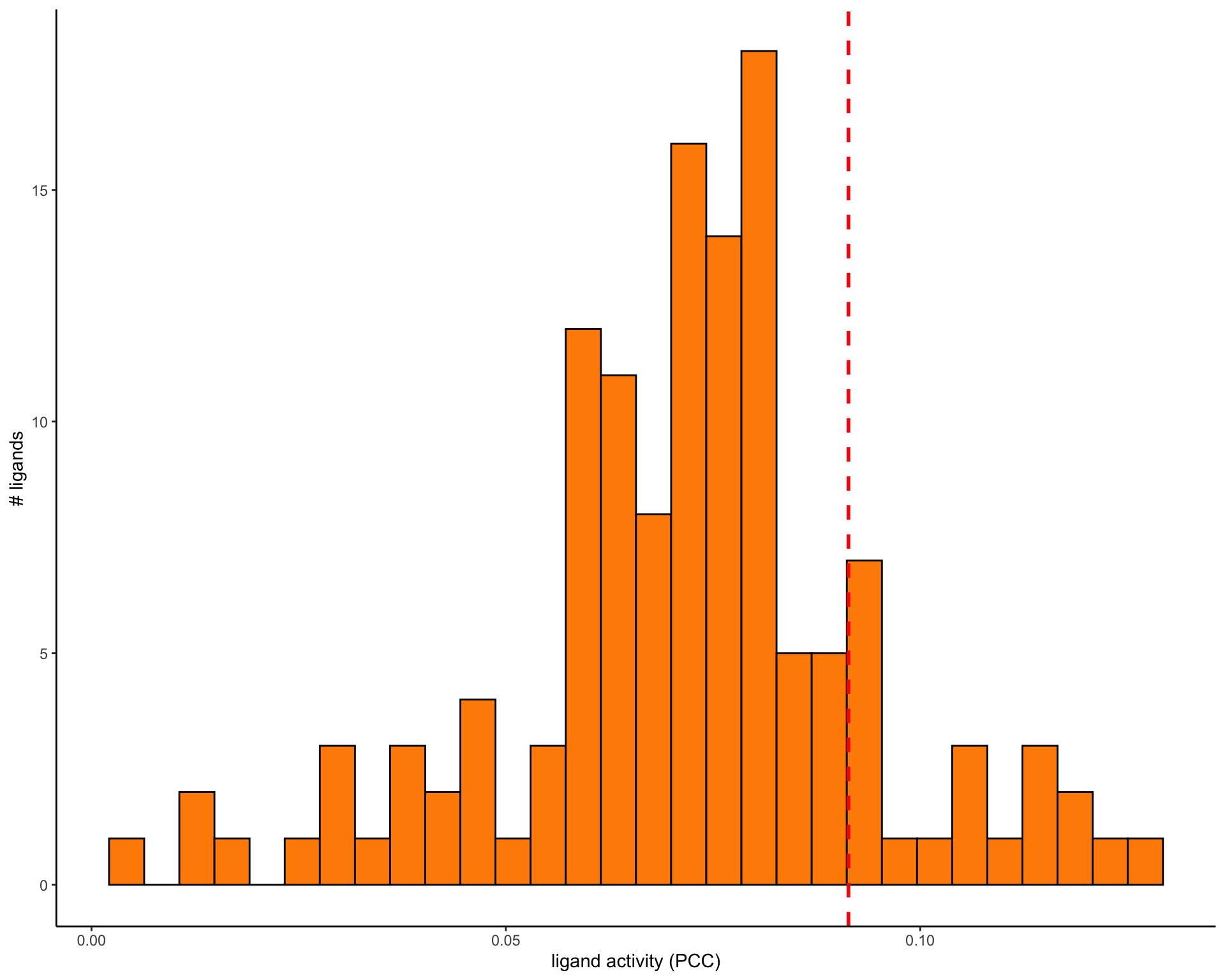

Past versions of activity-plot-1.png

Version	Author	Date
d3bd2d6	Luke Zappia	2020-05-27

Chunk time: 0.38 secs

6 Infer target genes

Once we have a set of active ligands we can look at the regulatory potential between ligands and downstream targets. We only look at interactions between the top 20 ligands and genes that belong to the gene set and are in the top 250 most strongly predicted targets of one of the selected ligands. The targets are selected based on predictions in the general prior model so are not specific to this dataset. Genes that are not a top target of one of the selected ligands will not be shown.

active_links <- best_ligands %>%
    lapply(
        get_weighted_ligand_target_links,
        geneset              = geneset,
        ligand_target_matrix = ligand_targets,
        n                    = 250
    ) %>%
    bind_rows()

skim(active_links)

Data summary

Name	active_links
Number of rows	143
Number of columns	3
_______________________
Column type frequency:
character	2
numeric	1
________________________
Group variables	None

Variable type: character

skim_variable	n_missing	complete_rate	min	max	empty	n_unique	whitespace
ligand	0	1	3	6	0	20	0
target	0	1	2	9	0	31	0

Variable type: numeric

skim_variable	n_missing	complete_rate	mean	sd	p0	p25	p50	p75	p100	hist
weight	0	1	0	0	0	0	0	0	0.01	▇▃▁▂▁

Chunk time: 0.18 secs

For visualisation potential scores are set to zero if they were below the 0.25 quantile for top targets of that ligand in the ligand-target matrix.

links_mat <- prepare_ligand_target_visualization(
    ligand_target_df     = active_links,
    ligand_target_matrix = ligand_targets,
    cutoff               = 0.25
)

order_ligands <- intersect(best_ligands, colnames(links_mat)) %>% rev()
order_targets <- active_links$target %>% unique()

vis_ligand_target <- links_mat[order_targets, order_ligands] %>% t()

ligand_target_heatmap <- vis_ligand_target %>%
    make_heatmap_ggplot(
        "Prioritized CAF-ligands",
        "p-EMT genes in malignant cells",
        color           = "purple",
        legend_position = "top",
        x_axis_position = "top",
        legend_title    = "Regulatory potential"
    ) +
    scale_fill_gradient2(
        low    = "whitesmoke",
        high   = "purple",
        breaks = c(0,0.005,0.01)
    ) +
    theme(axis.text.x = element_text(face = "italic"))

ligand_target_heatmap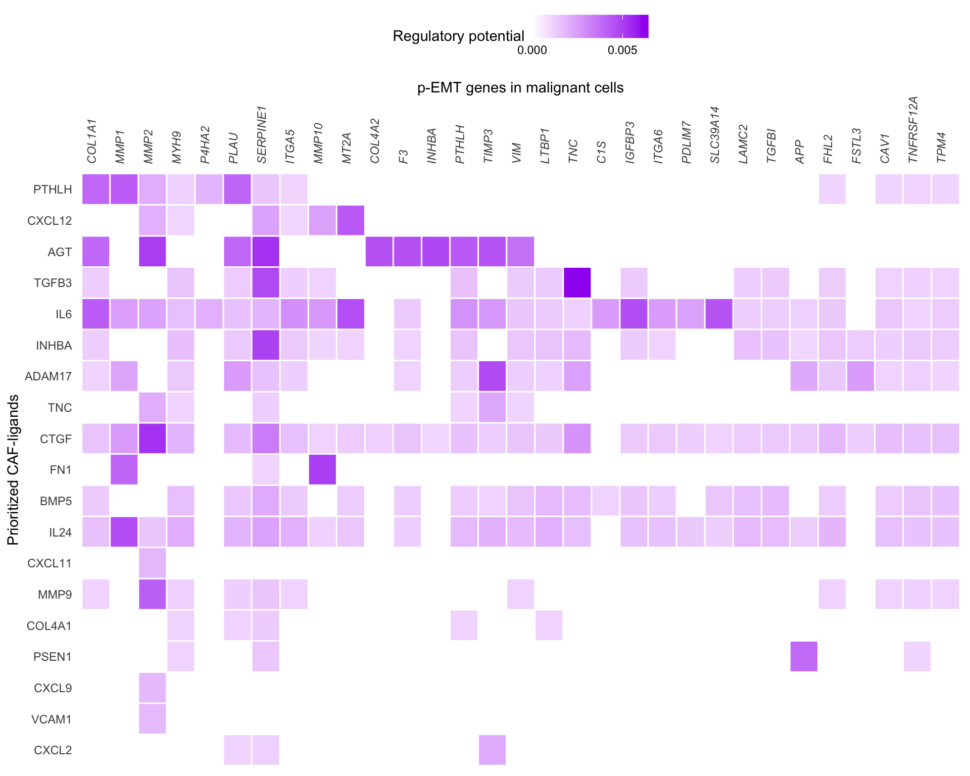

Past versions of target-heatmap-1.png

Version	Author	Date
d3bd2d6	Luke Zappia	2020-05-27

Chunk time: 0.98 secs

The cutoffs for visualisation are arbitary and the authors suggest testing several cutoffs. Considering more targets would identify more interactions but with less confidence. Lowering the quantil cutoff would result in a denser heatmap.

7 Ligand-receptor network

A further analysis is to look at the interactions between ligands and receptors rather than downstream targets.

lr_network_top <- lr_network %>%
    filter(
        from %in% best_ligands &
            to %in% expressed_receptors
    ) %>%
    distinct(from, to)

best_receptors <- lr_network_top %>%
    pull(to) %>%
    unique()

lr_network_top <- weighted_networks$lr_sig %>%
    filter(
        from %in% best_ligands &
            to %in% best_receptors
    ) %>%
    spread("from", "weight", fill = 0)

lr_network_top_mat <- lr_network_top %>%
    select(-to) %>%
    as.matrix() %>%
    magrittr::set_rownames(lr_network_top$to)

dist_receptors   <- dist(lr_network_top_mat, method = "binary")
hclust_receptors <- hclust(dist_receptors, method = "ward.D2")
order_receptors  <- hclust_receptors$labels[hclust_receptors$order]

dist_ligands            <- dist(lr_network_top_mat %>% t(), method = "binary")
hclust_ligands          <- hclust(dist_ligands, method = "ward.D2")
order_ligands_receptors <- hclust_ligands$labels[hclust_ligands$order]

ligand_receptor_heatmap <-
    lr_network_top_mat[order_receptors, order_ligands_receptors] %>%
    t() %>%
    make_heatmap_ggplot(
        "Prioritized CAF-ligands",
        "Receptors expressed by malignant cells",
        color           = "mediumvioletred",
        x_axis_position = "top",
        legend_title    = "Prior interaction potential"
    ) +
    theme()

ligand_receptor_heatmap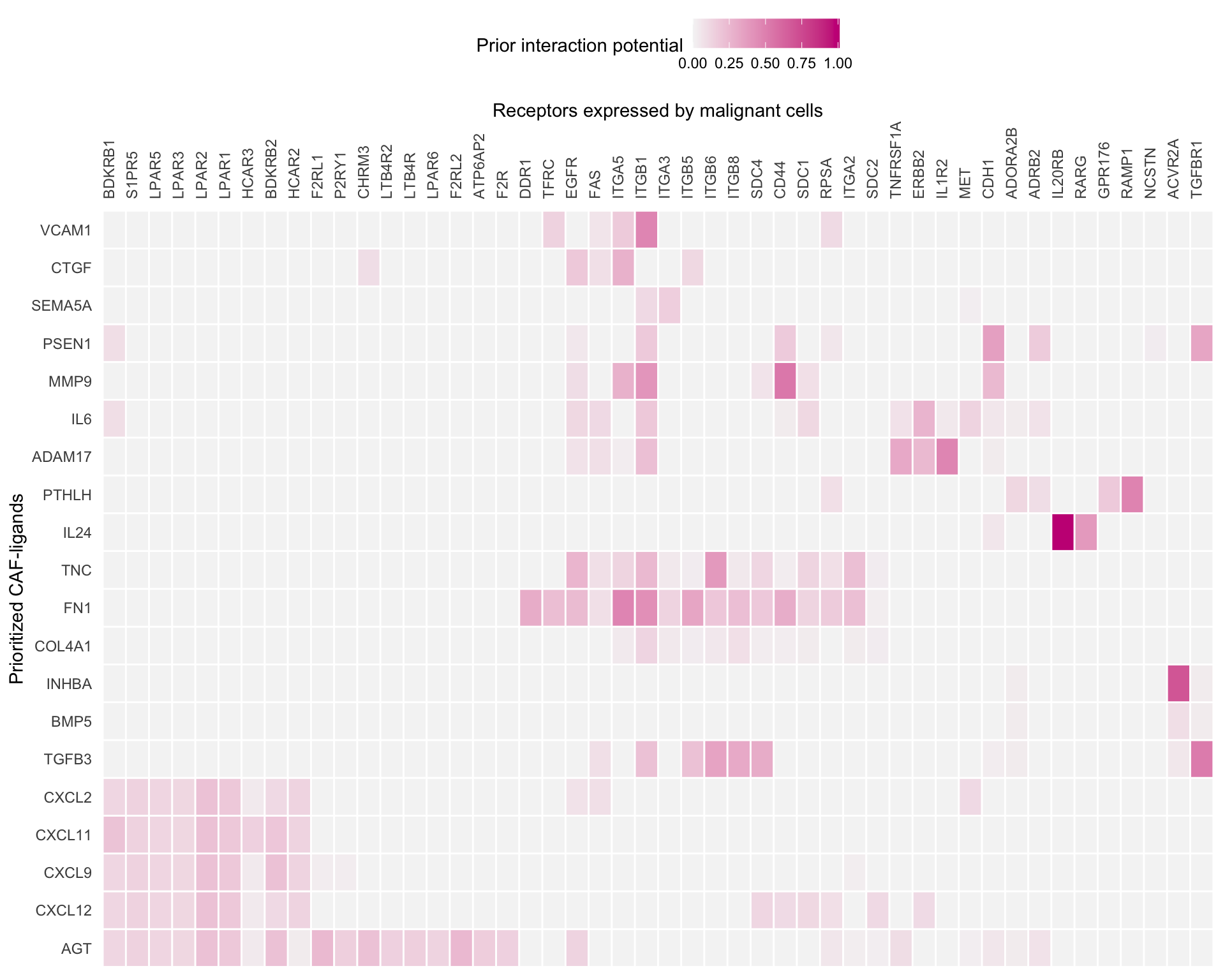

Past versions of lr-network-1.png

Version	Author	Date
d3bd2d6	Luke Zappia	2020-05-27

Chunk time: 0.87 secs

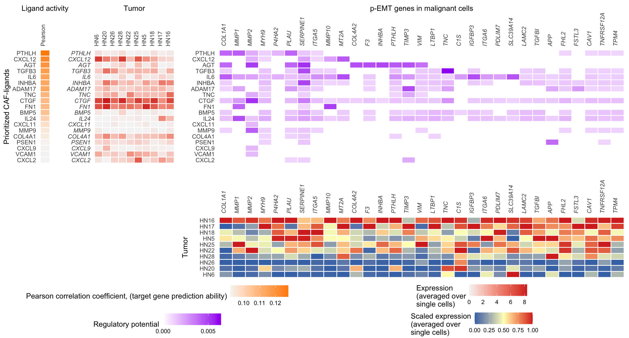
8 Combined heatmap (with expression)

NicheNet only considers expressed ligands but does not use their expression when ranking them, the ranking is only based on potential for regulation given prior knowledge. Here we make a combined heatmap that shows expression alongside regulatory potential.

ligand_pearson_matrix <- ligand_activities %>%
    select(pearson) %>%
    as.matrix() %>%
    magrittr::set_rownames(ligand_activities$test_ligand)

ligand_pearson_heatmap <- ligand_pearson_matrix[order_ligands, ] %>%
    as.matrix(ncol = 1) %>%
    magrittr::set_colnames("Pearson") %>%
    make_heatmap_ggplot(
        "Prioritized CAF-ligands",
        "Ligand activity",
        color           = "darkorange",
        legend_position = "top",
        x_axis_position = "top",
        legend_title    = paste(
            "Pearson correlation coefficient,",
            "(target gene prediction ability)",
            collapse = "\n"
        )
    )

expression_CAF <- exprs_mat[CAF_ids, order_ligands] %>%
    data.frame() %>%
    rownames_to_column("cell") %>%
    tbl_df() %>%
    inner_join(
        sample_info %>%
            select(cell,tumor),
        by =  "cell"
    ) %>%
    group_by(tumor) %>%
    select(-cell) %>%
    summarise_all(mean) %>%
    gather("ligand", "exprs", -tumor) %>%
    spread(tumor, exprs)
    
expression_CAF_mat <- expression_CAF %>%
    select(-ligand) %>%
    as.matrix() %>%
    magrittr::set_rownames(expression_CAF$ligand)

order_tumors = c("HN6", "HN20", "HN26", "HN28", "HN22", "HN25", 
                 "HN5", "HN18", "HN17", "HN16")

color <- colorRampPalette(rev(brewer.pal(n = 7, name = "RdYlBu")))(100)

ligand_exprs_heatmap <- expression_CAF_mat[order_ligands, order_tumors] %>% 
    make_heatmap_ggplot(
        "Prioritized CAF-ligands",
        "Tumor",
        color           = color[100],
        legend_position = "top",
        x_axis_position = "top",
        legend_title    = "Expression\n(averaged over\nsingle cells)"
    ) +
    theme(axis.text.y = element_text(face = "italic"))

expression_targets <- exprs_mat[malignant_ids, geneset] %>%
    data.frame() %>%
    rownames_to_column("cell") %>%
    tbl_df() %>%
    inner_join(
        sample_info %>%
            select(cell, tumor),
        by =  "cell"
    ) %>%
    group_by(tumor) %>%
    select(-cell) %>%
    summarise_all(mean) %>%
    gather("target", "exprs", -tumor) %>%
    spread(tumor, exprs)

expression_targets_mat <- expression_targets %>%
    select(-target) %>%
    as.matrix() %>%
    magrittr::set_rownames(expression_targets$target)

targets_exprs_heatmap <- expression_targets_mat %>%
    t() %>%
    scale_quantile() %>%
    .[order_tumors, order_targets] %>%
    make_threecolor_heatmap_ggplot(
        "Tumor",
        "Target",
        low_color       = color[1],
        mid_color       = color[50],
        mid             = 0.5,
        high_color      = color[100],
        legend_position = "top",
        x_axis_position = "top" ,
        legend_title    = "Scaled expression\n(averaged over\nsingle cells)"
    ) +
    theme(axis.text.x = element_text(face = "italic"))

combined_heatmap <- plot_grid(
    ligand_pearson_heatmap +
        theme(
            legend.position = "none",
            axis.ticks      = element_blank(),
            axis.title.x    = element_text()
        ),
    ligand_exprs_heatmap +
        ylab("") +
        theme(
            legend.position = "none",
            axis.ticks      = element_blank(),
            axis.title.x    = element_text()
        ),
    ligand_target_heatmap +
        ylab("") +
        theme(
            legend.position = "none",
            axis.ticks      = element_blank()
        ), 
    NULL,
    NULL,
    targets_exprs_heatmap +
        xlab("") +
        theme(
            legend.position = "none",
            axis.ticks      = element_blank()
        ), 
    align       = "hv",
    nrow        = 2,
    rel_widths  = c(
        1 + 4.5,
        ncol(expression_CAF_mat),
        ncol(vis_ligand_target)
    ) - 2,
    rel_heights = c(
        length(order_ligands),
        nrow(t(expression_targets_mat)) + 3
    )
) 

legends <- plot_grid(
    as_ggplot(get_legend(ligand_pearson_heatmap)),
    as_ggplot(get_legend(ligand_exprs_heatmap)),
    as_ggplot(get_legend(ligand_target_heatmap)),
    as_ggplot(get_legend(targets_exprs_heatmap)),
    nrow  = 2,
    align = "h"
)

plot_grid(
    combined_heatmap, 
    legends, 
    rel_heights = c(10, 2),
    nrow        = 2,
    align       = "hv"
)

Past versions of combined-heatmap-1.png

Version	Author	Date
d3bd2d6	Luke Zappia	2020-05-27

Chunk time: 2.67 secs

9 Signalling paths

NicheNet can also be used to infer the signalling paths between a ligands and targets of interest. This is done by looking at which transcription factors regulating the target are most closely downstream of the ligand. The pathway is confirmed by looking at the signalling database.

ligands_sel <- "TGFB3"
targets_sel <- c("TGFBI", "LAMC2", "TNC")

signalling_path <- get_ligand_signaling_path(
    ligand_tf_matrix  = ligand_targets,
    ligands_all       = ligands_sel,
    targets_all       = targets_sel,
    weighted_networks = weighted_networks
)

# Normalise edge weights for visualisation
signalling_path_minmax     <- signalling_path
signalling_path_minmax$sig <- signalling_path_minmax$sig %>%
    mutate(weight = ((weight - min(weight)) /
                         (max(weight) - min(weight))) + 0.75)
signalling_path_minmax$gr  <- signalling_path_minmax$gr %>%
    mutate(weight = ((weight - min(weight)) /
                         (max(weight) - min(weight))) + 0.75)

graph_minmax <- diagrammer_format_signaling_graph(
    signaling_graph_list = signalling_path_minmax,
    ligands_all          = ligands_sel,
    targets_all          = targets_sel,
    sig_color            = "indianred",
    gr_color             = "steelblue"
)

DiagrammeR::render_graph(graph_minmax, layout = "tree")

Chunk time: 4.97 secs

We can also look at which data sources support the interactions in this network. Here are examples of the first few sources.

path_sources <- infer_supporting_datasources(
    signaling_graph_list = signalling_path,
    lr_network           = lr_network,
    sig_network          = sig_network,
    gr_network           = gr_network
)

kable(head(path_sources, n = 10))

from	to	source	database	layer
ESR1	TGFBI	harmonizome_CHEA	harmonizome_gr	regulatory
ESR1	TGFBI	HTRIDB	HTRIDB	regulatory
ESR1	TGFBI	harmonizome_GEO_TF	harmonizome_gr	regulatory
ESR1	TGFBI	harmonizome_GEO_GENE	harmonizome_gr	regulatory
ESR1	TGFBI	lr_pathwaycommons_controls_expression_of	pathwaycommons_expression	regulatory
ESR1	TNC	harmonizome_ENCODE	harmonizome_gr	regulatory
ESR1	TNC	HTRIDB	HTRIDB	regulatory
ESR1	TNC	harmonizome_GEO_TF	harmonizome_gr	regulatory
FOS	LAMC2	harmonizome_ENCODE	harmonizome_gr	regulatory
FOS	LAMC2	Remap_5	Remap	regulatory

Chunk time: 8.07 secs

10 Gene set prediction

NicheNet can also use the top-ranked ligands to predict whether a gene belongs to a gene set. This is done by training a random forest classification model that returns a probability for each gene.

k_folds  <- 3
n_rounds <- 2

pemt_predictions <- seq(n_rounds) %>%
    lapply(
        assess_rf_class_probabilities,
        folds                      = k_folds,
        geneset                    = geneset,
        background_expressed_genes = background_genes,
        ligands_oi                 = best_ligands,
        ligand_target_matrix       = ligand_targets
    )

Chunk time: 33.61 secs

This returns a list with 2 items. Here is a summary of the first item:

Data summary

Name	pemt_predictions[[1]]
Number of rows	6072
Number of columns	3
_______________________
Column type frequency:
character	1
logical	1
numeric	1
________________________
Group variables	None

Variable type: character

skim_variable	n_missing	complete_rate	min	max	empty	n_unique	whitespace
gene	0	1	2	13	0	6072	0

Variable type: logical

skim_variable	n_missing	complete_rate	mean	count
response	0	1	0.02	FAL: 5976, TRU: 96

Variable type: numeric

skim_variable	n_missing	complete_rate	mean	sd	p0	p25	p50	p75	p100	hist
prediction	0	1	0.02	0.04	0	0	0.01	0.02	0.63	▇▁▁▁▁

We can then evaluate how well the calculated probabilites match up with the gene set assignments.

prediction_performance <- pemt_predictions %>%
    lapply(classification_evaluation_continuous_pred_wrapper) %>%
    bind_rows() %>%
    mutate(round = seq(1:nrow(.)))

prediction_performance %>%
    summarise(
        AUROC   = mean(auroc),
        AUPR    = mean(aupr),
        Pearson = mean(pearson)
    ) %>%
    kable()

AUROC	AUPR	Pearson
0.7318148	0.0845526	0.1751712

prediction_performance_discrete <- pemt_predictions %>%
    lapply(calculate_fraction_top_predicted, quantile_cutoff = 0.95) %>%
    bind_rows() %>%
    ungroup() %>%
    mutate(round = rep(1:length(pemt_predictions), each = 2))

pemt_frac <- prediction_performance_discrete %>%
    filter(true_target) %>%
    .$fraction_positive_predicted %>%
    mean()

nonpemt_frac <- prediction_performance_discrete %>%
    filter(!true_target) %>%
    .$fraction_positive_predicted %>%
    mean()

prediction_performance_fisher <- pemt_predictions %>%
    lapply(calculate_fraction_top_predicted_fisher, quantile_cutoff = 0.95) %>%
    unlist() %>%
    mean()

Chunk time: 0.14 secs

We see that 26% of p-EMT genes are classified as being part of the geneset and 5% of non-p-EMT genes. A Fisher’s exact test gives us a p-value of 8.3865289^{-11}.

The following p-EMT genes were correctly predicted in every cross-validation round:

seq(length(pemt_predictions)) %>%
    lapply(get_top_predicted_genes, pemt_predictions) %>%
    reduce(full_join, by = c("gene", "true_target")) %>%
    filter(true_target) %>%
    kable()

gene	true_target	predicted_top_target_round1	predicted_top_target_round2
MMP1	TRUE	TRUE	TRUE
COL1A1	TRUE	TRUE	TRUE
F3	TRUE	TRUE	TRUE
MT2A	TRUE	TRUE	TRUE
PLAU	TRUE	TRUE	TRUE
MMP2	TRUE	TRUE	TRUE
IGFBP3	TRUE	TRUE	TRUE
MMP10	TRUE	TRUE	TRUE
TNC	TRUE	TRUE	TRUE
TPM1	TRUE	TRUE	TRUE
SERPINE1	TRUE	TRUE	TRUE
TIMP3	TRUE	TRUE	TRUE
PTHLH	TRUE	TRUE	TRUE
STON2	TRUE	TRUE	NA
GJA1	TRUE	TRUE	TRUE
DKK3	TRUE	TRUE	NA
CDH13	TRUE	TRUE	TRUE
THBS1	TRUE	TRUE	NA
COL17A1	TRUE	TRUE	NA
ANXA8L1	TRUE	TRUE	NA
COL4A2	TRUE	TRUE	TRUE
NAGK	TRUE	TRUE	TRUE
TNFRSF12A	TRUE	TRUE	NA
LAMA3	TRUE	TRUE	NA
TPM4	TRUE	TRUE	NA
LAMC2	TRUE	TRUE	TRUE
INHBA	TRUE	NA	TRUE
FSTL3	TRUE	NA	TRUE
P4HA2	TRUE	NA	TRUE
ITGB1	TRUE	NA	TRUE
ITGB6	TRUE	NA	TRUE

Chunk time: 0.03 secs

11 Single-cell ligand activities

So far we have considered ligand activities for cell types but it is also possible to calculate ligand activities for individual cells.

To reduce run time we only perform this analysis on a selection of 10 cells from a single tumour.

exprs_scaled <- exprs_mat %>%
    .[malignant_ids, background_genes] %>%
    scale_quantile()

malignant_hn5_ids <- sample_info %>%
    filter(tumor == "HN5") %>%
    filter(`Lymph node` == 0) %>%
    filter(`classified  as cancer cell` == 1) %>%
    .$cell %>%
    head(10)

sc_ligand_activities <- predict_single_cell_ligand_activities(
    cell_ids             = malignant_hn5_ids,
    expression_scaled    = exprs_scaled,
    ligand_target_matrix = ligand_targets,
    potential_ligands    = potential_ligands
)

Chunk time: 1.67 mins

Now that we have activities at the single-cell level they can be linked to other properties of cells. Here we score cells on their expression of the core p-EMT gene TGFBI. This is taken as a proxy for p-EMT activity and correlated with the calculated ligand activities. The correlation can be used to rank p-EMT inducing ligands.

cell_scores <- tibble(
    cell  = malignant_hn5_ids,
    score = exprs_scaled[malignant_hn5_ids, "TGFBI"]
)

sc_ligand_activities_norm <- normalize_single_cell_ligand_activities(
    sc_ligand_activities
)

correlations <- single_ligand_activity_score_regression(
    sc_ligand_activities_norm,
    cell_scores
)

skim(correlations)

Data summary

Name	correlations
Number of rows	131
Number of columns	13
_______________________
Column type frequency:
character	1
numeric	12
________________________
Group variables	None

Variable type: character

skim_variable	n_missing	complete_rate	min	max	empty	n_unique	whitespace
ligand	0	1	2	8	0	131	0

Variable type: numeric

skim_variable	n_missing	complete_rate	mean	sd	p0	p25	p50	p75	p100	hist
r_squared	0	1	0.08	0.10	0.00	0.01	0.04	0.12	0.45	▇▂▁▁▁
adj_r_squared	0	1	-0.04	0.11	-0.12	-0.12	-0.08	0.01	0.38	▇▂▁▁▁
f_statistic	0	1	0.80	1.19	0.00	0.07	0.33	1.05	6.52	▇▁▁▁▁
lm_coefficient_abs_t	0	1	0.70	0.56	0.00	0.26	0.58	1.02	2.55	▇▆▃▁▁
inverse_rmse	0	1	6.39	0.40	6.10	6.13	6.23	6.49	8.22	▇▂▁▁▁
reverse_aic	0	1	4.90	1.18	4.02	4.10	4.42	5.25	9.98	▇▂▁▁▁
reverse_bic	0	1	3.99	1.18	3.11	3.20	3.52	4.34	9.07	▇▂▁▁▁
inverse_mae	0	1	8.33	0.71	7.64	7.86	8.10	8.41	10.96	▇▂▁▁▁
pearson_log_pval	0	1	0.33	0.31	0.00	0.10	0.24	0.47	1.47	▇▃▂▁▁
spearman_log_pval	0	1	0.36	0.35	0.00	0.09	0.29	0.50	1.67	▇▃▁▁▁
pearson_regression	0	1	0.02	0.28	-0.67	-0.18	0.04	0.23	0.53	▂▅▇▇▅
spearman_regression	0	1	0.00	0.30	-0.73	-0.22	0.02	0.24	0.60	▂▅▇▇▅

correlations %>%
    arrange(-pearson_regression) %>%
    select(ligand, pearson_regression) %>%
    head() %>%
    kable()

ligand	pearson_regression
TNC	0.5252682
TFPI	0.4974591
SEMA5A	0.4908069
ANXA1	0.4883174
TNFSF13B	0.4730668
IBSP	0.4615628

inner_join(cell_scores, sc_ligand_activities_norm) %>%
    ggplot(aes(score, TNC)) +
    geom_point() +
    geom_smooth(method = "lm")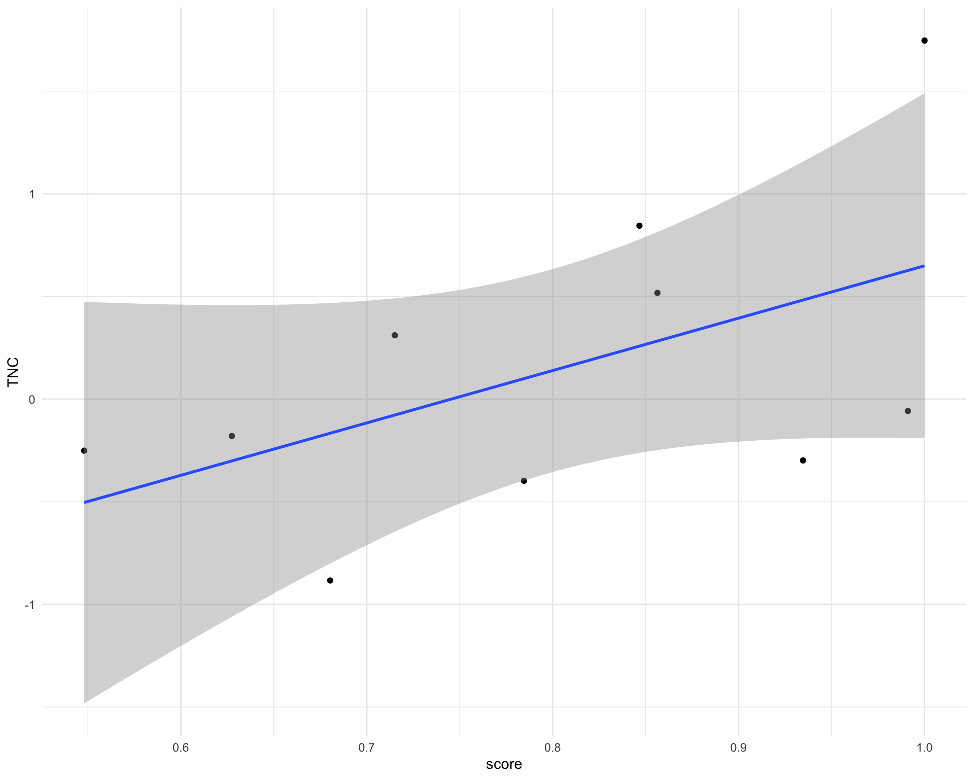

Past versions of score-cells-1.png

Version	Author	Date
d3bd2d6	Luke Zappia	2020-05-27

Chunk time: 1.23 secs

12 Circos plots

An alternative way to visualise interactions is using a Circos plot.

Summary

Parameters

This table describes parameters used and set in this document.

params <- list(
    
)
params <- toJSON(params, pretty = TRUE)
kable(fromJSON(params))

Chunk time: 0.01 secs

Output files

This table describes the output files produced by this document. Right click and Save Link As… to download the results.

write_tsv(ligand_activities, fs::path(OUT_DIR, "ligand_activities.tsv"))
write_tsv(active_links, fs::path(OUT_DIR, "active_links.tsv"))

kable(data.frame(
    File = c(
        download_link("parameters.json", OUT_DIR),
        download_link("ligand_activities.tsv", OUT_DIR),
        download_link("active_links.tsv", OUT_DIR)
    ),
    Description = c(
        "Parameters set and used in this analysis",
        "Ligand activites calculated by NicheNet",
        "Active links between ligands and targets inferred by NicheNet"
    )
))

File	Description
parameters.json	Parameters set and used in this analysis
ligand_activities.tsv	Ligand activites calculated by NicheNet
active_links.tsv	Active links between ligands and targets inferred by NicheNet

Chunk time: 0.2 secs

Session information

Session information

sessioninfo::session_info()

─ Session info ───────────────────────────────────────────────────────────────
 setting  value                       
 version  R version 4.0.0 (2020-04-24)
 os       macOS Catalina 10.15.7      
 system   x86_64, darwin17.0          
 ui       X11                         
 language (EN)                        
 collate  en_US.UTF-8                 
 ctype    en_US.UTF-8                 
 tz       Europe/Berlin               
 date     2020-11-24                  

─ Packages ───────────────────────────────────────────────────────────────────
 ! package       * version    date       lib
   abind           1.4-5      2016-07-21 [1]
   acepack         1.4.1      2016-10-29 [1]
 P assertthat      0.2.1      2019-03-21 [?]
 P backports       1.1.6      2020-04-05 [?]
 P base64enc       0.1-3      2015-07-28 [?]
 P base64url       1.4        2018-05-14 [?]
   bitops          1.0-6      2013-08-17 [1]
 P broom           0.5.6      2020-04-20 [?]
 P car             3.0-7      2020-03-11 [?]
 P carData         3.0-3      2019-11-16 [?]
   caret           6.0-86     2020-03-20 [1]
   caTools         1.18.0     2020-01-17 [1]
 P cellranger      1.1.0      2016-07-27 [?]
   checkmate       2.0.0      2020-02-06 [1]
 P circlize      * 0.4.9      2020-04-30 [?]
 P class           7.3-17     2020-04-26 [?]
 P cli             2.0.2      2020-02-28 [?]
 P cluster         2.1.0      2019-06-19 [?]
 P codetools       0.2-18     2020-11-04 [?]
 P colorspace      1.4-1      2019-03-18 [?]
 P conflicted    * 1.0.4      2019-06-21 [?]
 P cowplot       * 1.0.0      2019-07-11 [?]
 P crayon          1.3.4      2017-09-16 [?]
 P curl            4.3        2019-12-02 [?]
 P data.table      1.12.8     2019-12-09 [?]
 P DBI             1.1.0      2019-12-15 [?]
 P dbplyr          1.4.3      2020-04-19 [?]
 P DiagrammeR      1.0.5      2020-01-16 [?]
 P digest          0.6.25     2020-02-23 [?]
 P dplyr         * 0.8.5      2020-03-07 [?]
 P drake           7.12.0     2020-03-25 [?]
   e1071         * 1.7-3      2019-11-26 [1]
 P ellipsis        0.3.0      2019-09-20 [?]
 P evaluate        0.14       2019-05-28 [?]
 P fansi           0.4.1      2020-01-08 [?]
 P farver          2.0.3      2020-01-16 [?]
   fdrtool         1.2.15     2015-07-08 [1]
 P filelock        1.0.2      2018-10-05 [?]
 P forcats       * 0.5.0      2020-03-01 [?]
   foreach         1.5.0      2020-03-30 [1]
 P foreign         0.8-79     2020-04-26 [?]
   Formula         1.2-3      2018-05-03 [1]
 P fs            * 1.4.1      2020-04-04 [?]
 P generics        0.0.2      2018-11-29 [?]
 P ggplot2       * 3.3.0      2020-03-05 [?]
 P ggpubr        * 0.3.0      2020-05-04 [?]
   ggsignif        0.6.0      2019-08-08 [1]
 P git2r           0.27.1     2020-05-03 [?]
 P GlobalOptions   0.1.1      2019-09-30 [?]
 P glue          * 1.4.0      2020-04-03 [?]
 P gower           0.2.1      2019-05-14 [?]
   gridExtra       2.3        2017-09-09 [1]
 P gtable          0.3.0      2019-03-25 [?]
 P haven           2.2.0      2019-11-08 [?]
 P here          * 0.1        2017-05-28 [?]
 P highr           0.8        2019-03-20 [?]
   Hmisc           4.4-0      2020-03-23 [1]
 P hms             0.5.3      2020-01-08 [?]
 P htmlTable       1.13.3     2019-12-04 [?]
 P htmltools       0.5.0      2020-06-16 [?]
   htmlwidgets     1.5.1      2019-10-08 [1]
 P httpuv          1.5.2      2019-09-11 [?]
 P httr            1.4.1      2019-08-05 [?]
 P igraph          1.2.5      2020-03-19 [?]
   ipred           0.9-9      2019-04-28 [1]
   iterators       1.0.12     2019-07-26 [1]
   jpeg            0.1-8.1    2019-10-24 [1]
 P jsonlite      * 1.6.1      2020-02-02 [?]
 P knitr         * 1.28       2020-02-06 [?]
 P labeling        0.3        2014-08-23 [?]
 P later           1.0.0      2019-10-04 [?]
 P lattice         0.20-41    2020-04-02 [?]
   latticeExtra    0.6-29     2019-12-19 [1]
   lava            1.6.7      2020-03-05 [1]
 P lifecycle       0.2.0      2020-03-06 [?]
 P limma           3.44.1     2020-04-28 [?]
 P lubridate       1.7.8      2020-04-06 [?]
 P magrittr        1.5        2014-11-22 [?]
 P MASS            7.3-51.6   2020-04-26 [?]
 P Matrix          1.2-18     2019-11-27 [?]
 P memoise         1.1.0      2017-04-21 [?]
 P mgcv            1.8-31     2019-11-09 [?]
   ModelMetrics    1.2.2.2    2020-03-17 [1]
 P modelr          0.1.7      2020-04-30 [?]
 P munsell         0.5.0      2018-06-12 [?]
   nichenetr     * 0.1.0      2020-05-08 [1]
 P nlme            3.1-147    2020-04-13 [?]
 P nnet            7.3-14     2020-04-26 [?]
   openxlsx        4.1.5      2020-05-06 [1]
 P pander        * 0.6.3      2018-11-06 [?]
 P pillar          1.4.4      2020-05-05 [?]
 P pkgconfig       2.0.3      2019-09-22 [?]
 P plyr            1.8.6      2020-03-03 [?]
   png             0.1-7      2013-12-03 [1]
 P prettyunits     1.1.1      2020-01-24 [?]
   pROC            1.16.2     2020-03-19 [1]
   prodlim         2019.11.13 2019-11-17 [1]
 P progress        1.2.2      2019-05-16 [?]
 P promises        1.1.0      2019-10-04 [?]
 P purrr         * 0.3.4      2020-04-17 [?]
 P R6              2.4.1      2019-11-12 [?]
   randomForest    4.6-14     2018-03-25 [1]
 P RColorBrewer  * 1.1-2      2014-12-07 [?]
 P Rcpp            1.0.4.6    2020-04-09 [?]
 P readr         * 1.3.1      2018-12-21 [?]
 P readxl          1.3.1      2019-03-13 [?]
 P recipes         0.1.12     2020-05-01 [?]
 P renv            0.12.0     2020-08-28 [?]
 P repr            1.1.0      2020-01-28 [?]
 P reprex          0.3.0      2019-05-16 [?]
 P reshape2        1.4.4      2020-04-09 [?]
 P reticulate      1.16       2020-05-27 [?]
   rio             0.5.16     2018-11-26 [1]
 P rlang           0.4.6      2020-05-02 [?]
 P rmarkdown       2.1        2020-01-20 [?]
   ROCR            1.0-11     2020-05-02 [1]
 P rpart           4.1-15     2019-04-12 [?]
 P rprojroot       1.3-2      2018-01-03 [?]
 P rstatix         0.5.0      2020-04-28 [?]
 P rstudioapi      0.11       2020-02-07 [?]
 P rvest           0.3.5      2019-11-08 [?]
 P scales          1.1.0      2019-11-18 [?]
 P sessioninfo     1.1.1      2018-11-05 [?]
 P shape           1.4.4      2018-02-07 [?]
 P skimr         * 2.1.1      2020-04-16 [?]
 P storr           1.2.1      2018-10-18 [?]
 P stringi         1.4.6      2020-02-17 [?]
 P stringr       * 1.4.0      2019-02-10 [?]
 P survival        3.2-7      2020-09-28 [?]
 P tibble        * 3.0.1      2020-04-20 [?]
 P tidyr         * 1.0.3      2020-05-07 [?]
 P tidyselect      1.0.0      2020-01-27 [?]
 P tidyverse     * 1.3.0      2019-11-21 [?]
   timeDate        3043.102   2018-02-21 [1]
 P txtq            0.2.0      2019-10-15 [?]
 P vctrs           0.2.4      2020-03-10 [?]
   visNetwork      2.0.9      2019-12-06 [1]
 P whisker         0.4        2019-08-28 [?]
 P withr           2.2.0      2020-04-20 [?]
 P workflowr       1.6.2      2020-04-30 [?]
 P xfun            0.13       2020-04-13 [?]
 P xml2            1.3.2      2020-04-23 [?]
 P yaml            2.2.1      2020-02-01 [?]
   zip             2.0.4      2019-09-01 [1]
 source                             
 CRAN (R 4.0.0)                     
 CRAN (R 4.0.0)                     
 CRAN (R 4.0.0)                     
 CRAN (R 4.0.0)                     
 CRAN (R 4.0.0)                     
 standard (@1.4)                    
 CRAN (R 4.0.0)                     
 CRAN (R 4.0.0)                     
 CRAN (R 4.0.0)                     
 CRAN (R 4.0.0)                     
 CRAN (R 4.0.0)                     
 CRAN (R 4.0.0)                     
 standard (@1.1.0)                  
 CRAN (R 4.0.0)                     
 CRAN (R 4.0.0)                     
 CRAN (R 4.0.0)                     
 CRAN (R 4.0.0)                     
 CRAN (R 4.0.0)                     
 CRAN (R 4.0.2)                     
 standard (@1.4-1)                  
 standard (@1.0.4)                  
 CRAN (R 4.0.0)                     
 CRAN (R 4.0.0)                     
 CRAN (R 4.0.0)                     
 CRAN (R 4.0.1)                     
 CRAN (R 4.0.0)                     
 CRAN (R 4.0.0)                     
 CRAN (R 4.0.0)                     
 CRAN (R 4.0.0)                     
 CRAN (R 4.0.0)                     
 CRAN (R 4.0.0)                     
 CRAN (R 4.0.0)                     
 CRAN (R 4.0.0)                     
 standard (@0.14)                   
 CRAN (R 4.0.0)                     
 CRAN (R 4.0.0)                     
 CRAN (R 4.0.0)                     
 CRAN (R 4.0.0)                     
 CRAN (R 4.0.0)                     
 CRAN (R 4.0.0)                     
 CRAN (R 4.0.0)                     
 CRAN (R 4.0.0)                     
 CRAN (R 4.0.0)                     
 standard (@0.0.2)                  
 CRAN (R 4.0.0)                     
 CRAN (R 4.0.0)                     
 CRAN (R 4.0.0)                     
 CRAN (R 4.0.0)                     
 CRAN (R 4.0.0)                     
 CRAN (R 4.0.0)                     
 CRAN (R 4.0.0)                     
 CRAN (R 4.0.0)                     
 standard (@0.3.0)                  
 standard (@2.2.0)                  
 standard (@0.1)                    
 standard (@0.8)                    
 CRAN (R 4.0.0)                     
 CRAN (R 4.0.0)                     
 CRAN (R 4.0.0)                     
 CRAN (R 4.0.2)                     
 CRAN (R 4.0.0)                     
 standard (@1.5.2)                  
 standard (@1.4.1)                  
 CRAN (R 4.0.0)                     
 CRAN (R 4.0.0)                     
 CRAN (R 4.0.0)                     
 CRAN (R 4.0.0)                     
 CRAN (R 4.0.0)                     
 CRAN (R 4.0.0)                     
 standard (@0.3)                    
 standard (@1.0.0)                  
 CRAN (R 4.0.0)                     
 CRAN (R 4.0.0)                     
 CRAN (R 4.0.0)                     
 CRAN (R 4.0.0)                     
 Bioconductor                       
 CRAN (R 4.0.0)                     
 CRAN (R 4.0.0)                     
 CRAN (R 4.0.0)                     
 standard (@1.2-18)                 
 standard (@1.1.0)                  
 standard (@1.8-31)                 
 CRAN (R 4.0.0)                     
 CRAN (R 4.0.0)                     
 standard (@0.5.0)                  
 Github (saeyslab/nichenetr@e535b72)
 CRAN (R 4.0.0)                     
 CRAN (R 4.0.0)                     
 CRAN (R 4.0.0)                     
 CRAN (R 4.0.0)                     
 CRAN (R 4.0.0)                     
 CRAN (R 4.0.0)                     
 CRAN (R 4.0.0)                     
 CRAN (R 4.0.0)                     
 CRAN (R 4.0.0)                     
 CRAN (R 4.0.0)                     
 CRAN (R 4.0.0)                     
 CRAN (R 4.0.0)                     
 standard (@1.1.0)                  
 CRAN (R 4.0.0)                     
 CRAN (R 4.0.0)                     
 CRAN (R 4.0.0)                     
 standard (@1.1-2)                  
 CRAN (R 4.0.0)                     
 standard (@1.3.1)                  
 standard (@1.3.1)                  
 CRAN (R 4.0.0)                     
 CRAN (R 4.0.2)                     
 CRAN (R 4.0.0)                     
 standard (@0.3.0)                  
 CRAN (R 4.0.0)                     
 CRAN (R 4.0.2)                     
 CRAN (R 4.0.0)                     
 CRAN (R 4.0.0)                     
 CRAN (R 4.0.0)                     
 CRAN (R 4.0.0)                     
 CRAN (R 4.0.0)                     
 CRAN (R 4.0.0)                     
 CRAN (R 4.0.0)                     
 CRAN (R 4.0.0)                     
 standard (@0.3.5)                  
 standard (@1.1.0)                  
 CRAN (R 4.0.0)                     
 CRAN (R 4.0.0)                     
 CRAN (R 4.0.0)                     
 standard (@1.2.1)                  
 CRAN (R 4.0.0)                     
 CRAN (R 4.0.0)                     
 CRAN (R 4.0.2)                     
 CRAN (R 4.0.0)                     
 CRAN (R 4.0.0)                     
 CRAN (R 4.0.0)                     
 standard (@1.3.0)                  
 CRAN (R 4.0.0)                     
 standard (@0.2.0)                  
 CRAN (R 4.0.0)                     
 CRAN (R 4.0.0)                     
 standard (@0.4)                    
 CRAN (R 4.0.0)                     
 CRAN (R 4.0.0)                     
 CRAN (R 4.0.0)                     
 CRAN (R 4.0.0)                     
 CRAN (R 4.0.0)                     
 CRAN (R 4.0.0)                     

[1] /Users/luke.zappia/Documents/Projects/interaction-tools/renv/library/R-4.0/x86_64-apple-darwin17.0
[2] /private/var/folders/rj/60lhr791617422kqvh0r4vy40000gn/T/RtmpOqMPdA/renv-system-library
[3] /private/var/folders/rj/60lhr791617422kqvh0r4vy40000gn/T/RtmpqYMqtc/renv-system-library
[4] /private/var/folders/rj/60lhr791617422kqvh0r4vy40000gn/T/RtmpS7cMys/renv-system-library

 P ── Loaded and on-disk path mismatch.

Chunk time: 0.34 secs