talklr example

workflowr

• Summary
• Checks
• Past versions

Last updated: 2020-11-24

Checks: 7 0

Knit directory: interaction-tools/

This reproducible R Markdown analysis was created with workflowr (version 1.6.2). The Checks tab describes the reproducibility checks that were applied when the results were created. The Past versions tab lists the development history.

---

R Markdown file: up-to-date

Great! Since the R Markdown file has been committed to the Git repository, you know the exact version of the code that produced these results.

Environment: empty

Great job! The global environment was empty. Objects defined in the global environment can affect the analysis in your R Markdown file in unknown ways. For reproduciblity it’s best to always run the code in an empty environment.

Seed: set.seed(20191213)

The command set.seed(20191213) was run prior to running the code in the R Markdown file. Setting a seed ensures that any results that rely on randomness, e.g. subsampling or permutations, are reproducible.

Session information: recorded

Great job! Recording the operating system, R version, and package versions is critical for reproducibility.

Cache: none

Nice! There were no cached chunks for this analysis, so you can be confident that you successfully produced the results during this run.

File paths: relative

Great job! Using relative paths to the files within your workflowr project makes it easier to run your code on other machines.

Repository version: 0333fe3

Great! You are using Git for version control. Tracking code development and connecting the code version to the results is critical for reproducibility.

The results in this page were generated with repository version 0333fe3. See the Past versions tab to see a history of the changes made to the R Markdown and HTML files.

Note that you need to be careful to ensure that all relevant files for the analysis have been committed to Git prior to generating the results (you can use wflow_publish or wflow_git_commit). workflowr only checks the R Markdown file, but you know if there are other scripts or data files that it depends on. Below is the status of the Git repository when the results were generated:

Ignored files:
    Ignored:    .Rhistory
    Ignored:    .Rproj.user/
    Ignored:    .drake/
    Ignored:    data/COMUNET/
    Ignored:    data/CellChat/
    Ignored:    data/ICELLNET/
    Ignored:    data/NicheNet/
    Ignored:    data/cellphonedb/
    Ignored:    data/celltalker/
    Ignored:    output/14-CellChat.Rmd/
    Ignored:    output/15-talklr.Rmd/
    Ignored:    output/16-CiteFuse.Rmd/
    Ignored:    output/17-scTHI.Rmd/
    Ignored:    output/18-celltalker.Rmd/
    Ignored:    output/index.Rmd/
    Ignored:    renv/library/
    Ignored:    renv/python/
    Ignored:    renv/staging/

Unstaged changes:
    Modified:   _drake.R

Note that any generated files, e.g. HTML, png, CSS, etc., are not included in this status report because it is ok for generated content to have uncommitted changes.

---

These are the previous versions of the repository in which changes were made to the R Markdown (analysis/15-talklr.Rmd) and HTML (docs/15-talklr.html) files. If you’ve configured a remote Git repository (see ?wflow_git_remote), click on the hyperlinks in the table below to view the files as they were in that past version.

File	Version	Author	Date	Message
html	9940762	Luke Zappia	2020-09-24	Add talklr to drake
Rmd	c67cf07	Luke Zappia	2020-09-24	Add talklr example
html	c67cf07	Luke Zappia	2020-09-24	Add talklr example
Rmd	d6b5957	Luke Zappia	2020-09-24	Set up talklr document
html	d6b5957	Luke Zappia	2020-09-24	Set up talklr document

---

# Setup document
source(here::here("code", "setup.R"))

# Function dependencies
invisible(drake::readd(download_link))

Introduction

In this document we are going to run through the example analysis for the talklr package and have a look at the output it produces. More information about talklr can be found at https://github.com/yuliangwang/talklr.

library("talklr")
library("dplyr")

Chunk time: 0.09 secs

1 Input

1.1 Mean expression

The main input to talklr is a data.frame with mean expression values for each cell type. These should be normalised for sequencing depth but not gene length and must not be log-transformed.

expr <- read.table(
    system.file(
        "extdata", "glom_normal_data.txt",
        package = "talklr"
    ),
    header = TRUE,
    sep    = "\t"
)

skim(expr)

Data summary

Name	expr
Number of rows	49947
Number of columns	4
_______________________
Column type frequency:
character	1
numeric	3
________________________
Group variables	None

Variable type: character

skim_variable	n_missing	complete_rate	min	max	empty	n_unique	whitespace
genes	0	1	0	16	1753	48037	0

Variable type: numeric

skim_variable	n_missing	complete_rate	mean	sd	p0	p25	p50	p75	p100	hist
podo	0	1	19.93	1288.81	0	0	0.01	2.79	226195.4	▇▁▁▁▁
mesa	0	1	19.91	1176.52	0	0	0.10	3.86	203422.4	▇▁▁▁▁
endo	0	1	19.92	1399.89	0	0	0.11	3.21	238898.1	▇▁▁▁▁

Chunk time: 0.32 secs

There is also a second example dataset from another condition.

expr_fsgs <- read.table(
    system.file(
        "extdata", "glom_fsgs_data.txt",
        package = "talklr"
    ),
    header = TRUE,
    sep    = "\t"
)

skim(expr_fsgs)

Data summary

Name	expr_fsgs
Number of rows	49947
Number of columns	4
_______________________
Column type frequency:
character	1
numeric	3
________________________
Group variables	None

Variable type: character

skim_variable	n_missing	complete_rate	min	max	empty	n_unique	whitespace
genes	0	1	0	16	1753	48037	0

Variable type: numeric

skim_variable	n_missing	complete_rate	mean	sd	p0	p25	p50	p75	p100	hist
podo	0	1	19.95	1695.24	0	0	0.03	2.63	308256.7	▇▁▁▁▁
mesa	0	1	19.93	1569.87	0	0	0.15	3.01	272528.5	▇▁▁▁▁
endo	0	1	19.92	1497.73	0	0	0.10	3.22	235597.0	▇▁▁▁▁

Chunk time: 0.34 secs

1.2 Database

A ligand-receptor database is included as part of the talklr package. This is used automatically during the analysis.

skim(talklr::receptor_ligand)

Data summary

Name	talklr::receptor_ligand
Number of rows	2422
Number of columns	16
_______________________
Column type frequency:
character	16
________________________
Group variables	None

Variable type: character

skim_variable	n_missing	complete_rate	min	max	empty	n_unique	whitespace
Pair.Name	0	1.00	5	18	0	2422	0
Ligand.ApprovedSymbol	0	1.00	2	9	0	695	0
Ligand.Name	0	1.00	5	139	0	695	0
Receptor.ApprovedSymbol	0	1.00	2	9	0	652	0
Receptor.Name	0	1.00	7	101	0	652	0
DLRP	1957	0.19	4	4	0	1	0
HPMR	1596	0.34	4	4	0	1	0
IUPHAR	2067	0.15	6	6	0	1	0
HPRD	1154	0.52	4	4	0	1	0
STRING.binding	1113	0.54	14	14	0	1	0
STRING.experiment	2003	0.17	17	17	0	1	0
HPMR.Ligand	567	0.77	2	8	0	458	0
HPMR.Receptor	310	0.87	2	9	0	505	0
PMID.Manual	2149	0.11	6	18	0	185	0
Pair.Source	0	1.00	5	5	0	2	0
Pair.Evidence	0	1.00	8	20	0	2	0

Chunk time: 0.28 secs

2 Single condition

2.1 Build network

The first step in a talklr analysis is to construct a network of ligand-receptor interactions and prioritise them using Kullback-Leibler divergence. The output is a data.frame with the ligand-receptor pairs, their expression in different cell types and the KL score.

lr_net <- make_expressed_net(
    expr,
    expressed_thresh = 4,
    receptor_ligand,
    KL_method = "product",
    pseudo_count = 1
)
lr_net <- arrange(lr_net, desc(KL))

skim(lr_net)

Data summary

Name	lr_net
Number of rows	652
Number of columns	23
_______________________
Column type frequency:
character	16
numeric	7
________________________
Group variables	None

Variable type: character

skim_variable	n_missing	complete_rate	min	max	empty	n_unique	whitespace
Pair.Name	0	1.00	7	17	0	652	0
Ligand.ApprovedSymbol	0	1.00	2	8	0	199	0
Ligand.Name	0	1.00	5	112	0	199	0
Receptor.ApprovedSymbol	0	1.00	2	9	0	197	0
Receptor.Name	0	1.00	7	92	0	197	0
DLRP	534	0.18	4	4	0	1	0
HPMR	457	0.30	4	4	0	1	0
IUPHAR	620	0.05	6	6	0	1	0
HPRD	335	0.49	4	4	0	1	0
STRING.binding	255	0.61	14	14	0	1	0
STRING.experiment	536	0.18	17	17	0	1	0
HPMR.Ligand	159	0.76	2	8	0	137	0
HPMR.Receptor	67	0.90	2	9	0	164	0
PMID.Manual	568	0.13	7	18	0	70	0
Pair.Source	0	1.00	5	5	0	2	0
Pair.Evidence	0	1.00	8	20	0	2	0

Variable type: numeric

skim_variable	n_missing	complete_rate	mean	sd	p0	p25	p50	p75	p100	hist
ligand_podo	0	1	110.11	324.72	1.00	2.76	6.39	61.24	1806.63	▇▁▁▁▁
ligand_mesa	0	1	139.25	642.01	1.02	5.54	22.80	69.78	10226.73	▇▁▁▁▁
ligand_endo	0	1	100.74	759.82	1.00	2.76	13.21	52.53	13475.95	▇▁▁▁▁
receptor_podo	0	1	130.63	306.47	1.00	3.04	12.03	92.05	2099.77	▇▁▁▁▁
receptor_mesa	0	1	151.43	283.86	1.00	8.65	32.30	151.70	1971.31	▇▁▁▁▁
receptor_endo	0	1	120.88	218.35	1.00	3.58	20.48	105.59	1202.78	▇▁▁▁▁
KL	0	1	1.29	0.61	0.01	0.81	1.29	1.72	2.90	▃▇▇▅▁

Chunk time: 0.21 secs

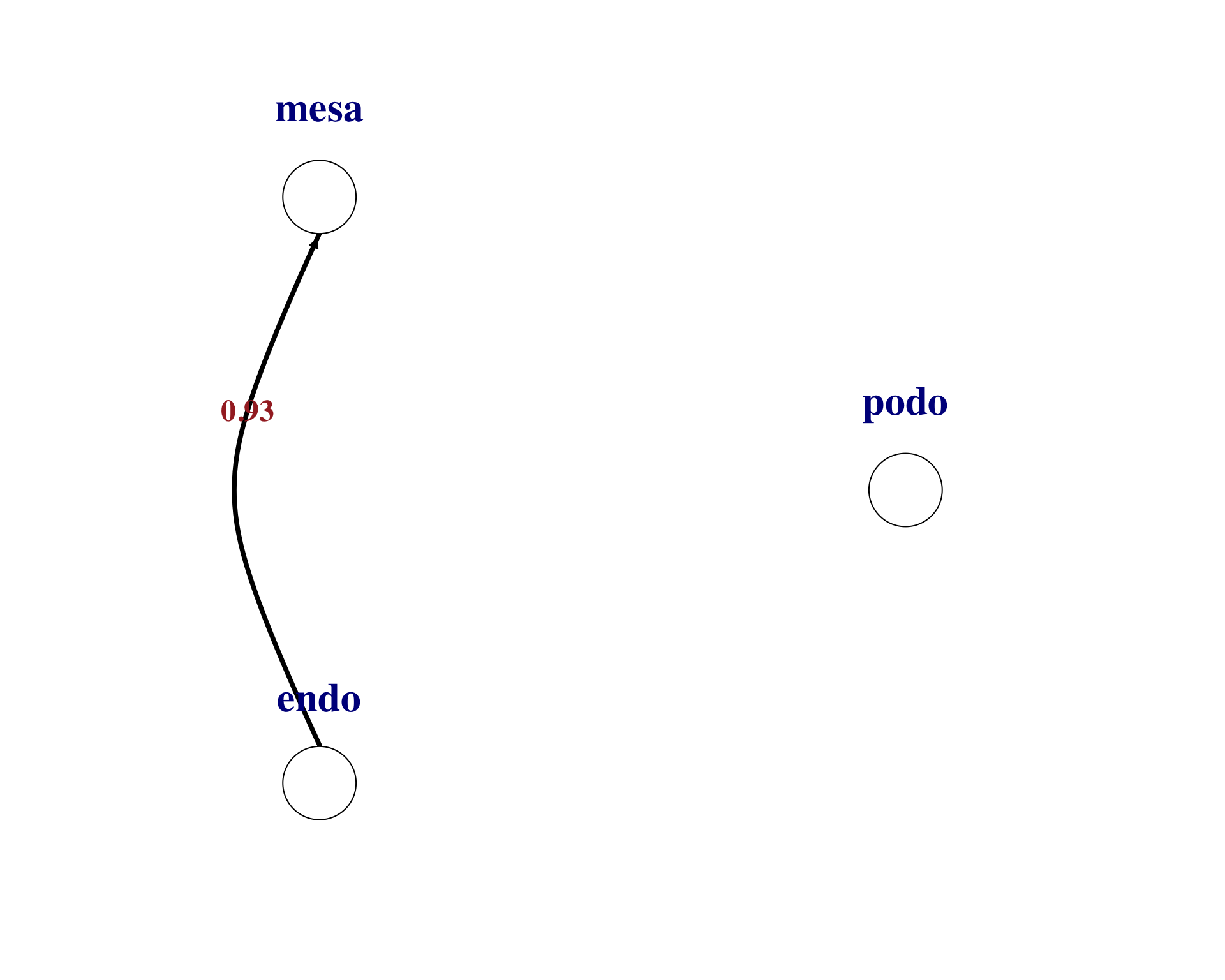
2.2 Visualise pairs

We can then visualise individual ligand-receptor pair interactions between cell types. Here are examples for the top two pairs.

plot_lr_wiring(
    ligand_exprs   = as.numeric(lr_net[1, 17:19]),
    receptor_exprs = as.numeric(lr_net[1, 20:22]),
    cell_labels    = c("podo","mesa","endo"),
    thresh         = 0
)

Past versions of single-vis-1.png

Version	Author	Date
c67cf07	Luke Zappia	2020-09-24

plot_lr_wiring(
    ligand_exprs   = as.numeric(lr_net[2, 17:19]),
    receptor_exprs = as.numeric(lr_net[2, 20:22]),
    cell_labels    = c("podo","mesa","endo"),
    thresh         = 0
)

Past versions of single-vis-2.png

Version	Author	Date
c67cf07	Luke Zappia	2020-09-24

Chunk time: 0.27 secs

2.3 DEG method

Testing for differential expression can be used to select those pairs where both the ligand and receptor are “marker” genes for a cell type.

lr_net_deg <- make_deg_net(
    expr,
    lr_net,
    fc_thresh    = 3,
    pseudo_count = 1
)

Chunk time: 0.07 secs

There are 198 pairs selected using this method.

3 Two conditions

There is another mode in talklr that lets us compare between conditions.

3.1 Gene selection

First we select genes that are expressed in at least one cell type in at least one of the conditions. We set a threshold of at least 4 in at least 1 cell type.

expressed_norm <- rowSums(expr[, 2:ncol(expr)] > 4) >= 1
expressed_fsgs <- rowSums(expr_fsgs[, 2:ncol(expr_fsgs)] > 4) >= 1
expressed_genes <- expr$genes[expressed_norm | expressed_fsgs]

Chunk time: 0.01 secs

3.2 Build networks

We then build a network for each condition.

norm_net <- make_expressed_net_specify_expressed_genes(
    expr,
    expressed_genes,
    receptor_ligand,
    KL_method = "product"
)

fsgs_net <- make_expressed_net_specify_expressed_genes(
    expr_fsgs,
    expressed_genes,
    receptor_ligand,
    KL_method = "product"
)

Chunk time: 0.07 secs

3.3 Compare conditions

Once we have the two conditions we can compare them to look at the differences. The result from this is similar to what we get for a single condition but with an extra column scoring the difference.

norm_net$fsgs_vs_norm_KL <- disease_vs_normal_KL(
    fsgs_net[, 17:19],
    fsgs_net[, 20:22],
    norm_net[, 17:19],
    norm_net[, 20:22],
    pseudo_count = 1,
    method = "product"
)

perturbed_net <- arrange(norm_net, desc(fsgs_vs_norm_KL))

skim(perturbed_net)

Data summary

Name	perturbed_net
Number of rows	722
Number of columns	24
_______________________
Column type frequency:
character	16
numeric	8
________________________
Group variables	None

Variable type: character

skim_variable	n_missing	complete_rate	min	max	empty	n_unique	whitespace
Pair.Name	0	1.00	7	17	0	722	0
Ligand.ApprovedSymbol	0	1.00	2	8	0	215	0
Ligand.Name	0	1.00	5	112	0	215	0
Receptor.ApprovedSymbol	0	1.00	2	9	0	208	0
Receptor.Name	0	1.00	7	92	0	208	0
DLRP	595	0.18	4	4	0	1	0
HPMR	505	0.30	4	4	0	1	0
IUPHAR	689	0.05	6	6	0	1	0
HPRD	372	0.48	4	4	0	1	0
STRING.binding	280	0.61	14	14	0	1	0
STRING.experiment	600	0.17	17	17	0	1	0
HPMR.Ligand	172	0.76	2	8	0	148	0
HPMR.Receptor	71	0.90	2	9	0	174	0
PMID.Manual	628	0.13	7	18	0	79	0
Pair.Source	0	1.00	5	5	0	2	0
Pair.Evidence	0	1.00	8	20	0	2	0

Variable type: numeric

skim_variable	n_missing	complete_rate	mean	sd	p0	p25	p50	p75	p100	hist
ligand_podo	0	1	103.22	314.37	0.00	1.45	4.79	51.30	1805.63	▇▁▁▁▁
ligand_mesa	0	1	131.91	622.02	0.02	3.30	18.80	64.58	10225.73	▇▁▁▁▁
ligand_endo	0	1	96.06	730.41	0.00	1.72	9.95	41.85	13474.95	▇▁▁▁▁
receptor_podo	0	1	124.31	299.07	0.00	1.83	10.76	80.65	2098.77	▇▁▁▁▁
receptor_mesa	0	1	145.25	284.35	0.00	5.14	26.34	150.70	1970.31	▇▁▁▁▁
receptor_endo	0	1	114.67	216.12	0.00	2.43	15.85	99.10	1201.78	▇▁▁▁▁
KL	0	1	1.47	0.68	0.01	0.99	1.45	1.95	2.96	▃▅▇▅▂
fsgs_vs_norm_KL	0	1	0.13	0.13	0.00	0.06	0.10	0.17	1.55	▇▁▁▁▁

Chunk time: 0.18 secs

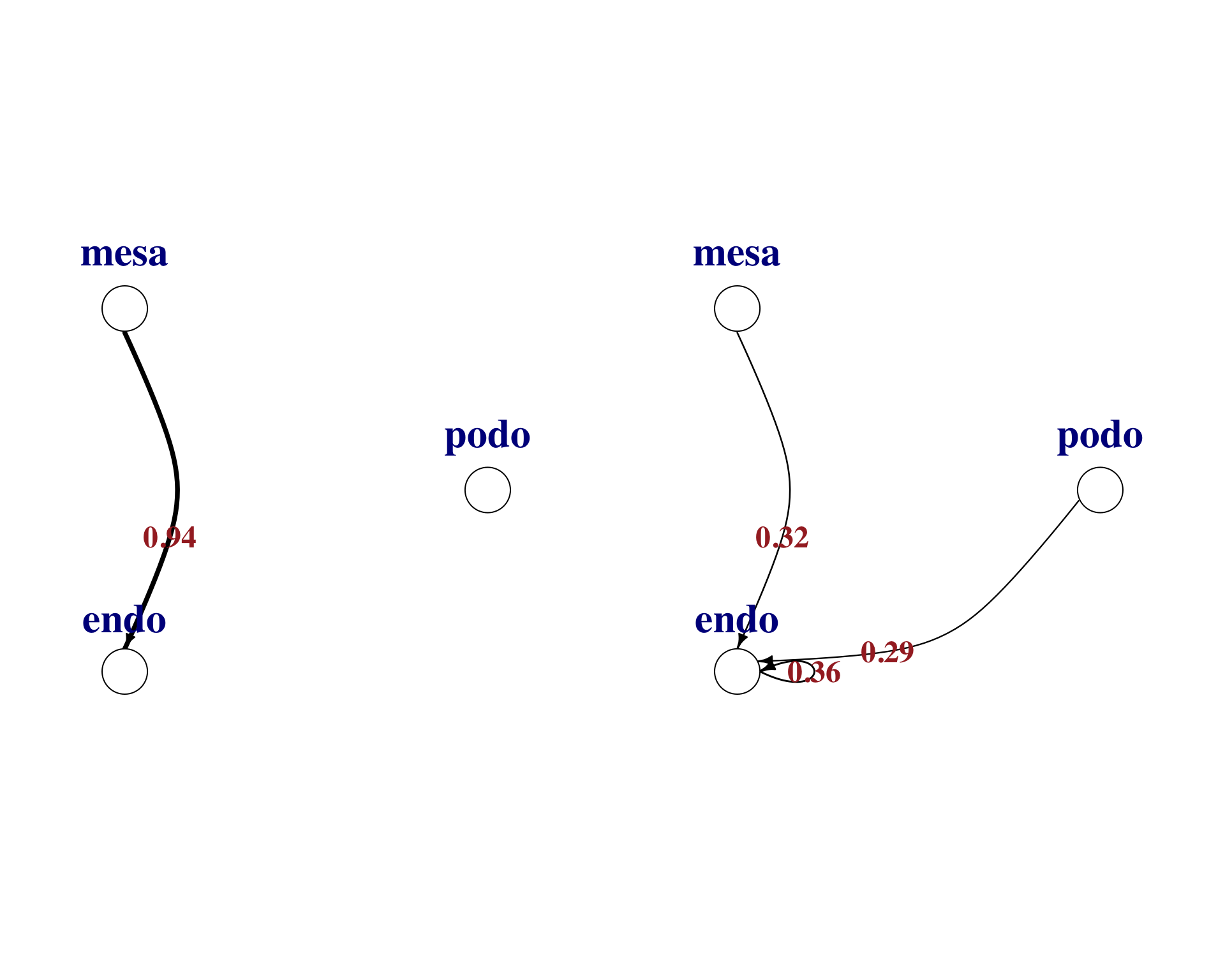
3.4 Visualise differences

We can use the same plotting function to visualise the differences between the conditions.

pair <- "CCL2_ACKR2"

par(mfrow = c(1,2))
par(mar = c(0.3, 0.3, 0.3, 0.3))

plot_lr_wiring(
    ligand_exprs   = as.numeric(norm_net[norm_net$Pair.Name == pair, 17:19]),
    receptor_exprs = as.numeric(norm_net[norm_net$Pair.Name == pair, 20:22]),
    cell_labels    = c("podo","mesa","endo"),
    thresh         = 0
) 

plot_lr_wiring(
    ligand_exprs   = as.numeric(fsgs_net[fsgs_net$Pair.Name == pair, 17:19]),
    receptor_exprs = as.numeric(fsgs_net[fsgs_net$Pair.Name == pair, 20:22]),
    cell_labels    = c("podo","mesa","endo"),
    thresh         = 0
)

Past versions of two-vis-1.png

Version	Author	Date
c67cf07	Luke Zappia	2020-09-24

Chunk time: 0.12 secs

Summary

Parameters

This table describes parameters used and set in this document.

params <- list(
    
)
params <- toJSON(params, pretty = TRUE)
kable(fromJSON(params))

Chunk time: 0.01 secs

Output files

This table describes the output files produced by this document. Right click and Save Link As… to download the results.

kable(data.frame(
    File = c(
        download_link("parameters.json", OUT_DIR)
    ),
    Description = c(
        "Parameters set and used in this analysis"
    )
))

File	Description
parameters.json	Parameters set and used in this analysis

Chunk time: 0.01 secs

Session information

Session information

sessioninfo::session_info()

─ Session info ───────────────────────────────────────────────────────────────
 setting  value                       
 version  R version 4.0.0 (2020-04-24)
 os       macOS Catalina 10.15.7      
 system   x86_64, darwin17.0          
 ui       X11                         
 language (EN)                        
 collate  en_US.UTF-8                 
 ctype    en_US.UTF-8                 
 tz       Europe/Berlin               
 date     2020-11-24                  

─ Packages ───────────────────────────────────────────────────────────────────
 ! package     * version    date       lib source                             
 P assertthat    0.2.1      2019-03-21 [?] CRAN (R 4.0.0)                     
 P backports     1.1.6      2020-04-05 [?] CRAN (R 4.0.0)                     
 P base64enc     0.1-3      2015-07-28 [?] CRAN (R 4.0.0)                     
 P base64url     1.4        2018-05-14 [?] standard (@1.4)                    
 P broom         0.5.6      2020-04-20 [?] CRAN (R 4.0.0)                     
 P cellranger    1.1.0      2016-07-27 [?] standard (@1.1.0)                  
 P cli           2.0.2      2020-02-28 [?] CRAN (R 4.0.0)                     
 P colorspace    1.4-1      2019-03-18 [?] standard (@1.4-1)                  
 P conflicted  * 1.0.4      2019-06-21 [?] standard (@1.0.4)                  
 P crayon        1.3.4      2017-09-16 [?] CRAN (R 4.0.0)                     
 P DBI           1.1.0      2019-12-15 [?] CRAN (R 4.0.0)                     
 P dbplyr        1.4.3      2020-04-19 [?] CRAN (R 4.0.0)                     
 P digest        0.6.25     2020-02-23 [?] CRAN (R 4.0.0)                     
 P dplyr       * 0.8.5      2020-03-07 [?] CRAN (R 4.0.0)                     
 P drake         7.12.0     2020-03-25 [?] CRAN (R 4.0.0)                     
 P ellipsis      0.3.0      2019-09-20 [?] CRAN (R 4.0.0)                     
 P evaluate      0.14       2019-05-28 [?] standard (@0.14)                   
 P fansi         0.4.1      2020-01-08 [?] CRAN (R 4.0.0)                     
 P filelock      1.0.2      2018-10-05 [?] CRAN (R 4.0.0)                     
 P forcats     * 0.5.0      2020-03-01 [?] CRAN (R 4.0.0)                     
 P fs          * 1.4.1      2020-04-04 [?] CRAN (R 4.0.0)                     
 P generics      0.0.2      2018-11-29 [?] standard (@0.0.2)                  
 P ggplot2     * 3.3.0      2020-03-05 [?] CRAN (R 4.0.0)                     
 P git2r         0.27.1     2020-05-03 [?] CRAN (R 4.0.0)                     
 P glue        * 1.4.0      2020-04-03 [?] CRAN (R 4.0.0)                     
 P gtable        0.3.0      2019-03-25 [?] standard (@0.3.0)                  
 P haven         2.2.0      2019-11-08 [?] standard (@2.2.0)                  
 P here        * 0.1        2017-05-28 [?] standard (@0.1)                    
 P highr         0.8        2019-03-20 [?] standard (@0.8)                    
 P hms           0.5.3      2020-01-08 [?] CRAN (R 4.0.0)                     
 P htmltools     0.5.0      2020-06-16 [?] CRAN (R 4.0.2)                     
 P httpuv        1.5.2      2019-09-11 [?] standard (@1.5.2)                  
 P httr          1.4.1      2019-08-05 [?] standard (@1.4.1)                  
 P igraph      * 1.2.5      2020-03-19 [?] CRAN (R 4.0.0)                     
 P jsonlite    * 1.6.1      2020-02-02 [?] CRAN (R 4.0.0)                     
 P knitr       * 1.28       2020-02-06 [?] CRAN (R 4.0.0)                     
 P later         1.0.0      2019-10-04 [?] standard (@1.0.0)                  
 P lattice       0.20-41    2020-04-02 [?] CRAN (R 4.0.0)                     
 P lifecycle     0.2.0      2020-03-06 [?] CRAN (R 4.0.0)                     
 P lubridate     1.7.8      2020-04-06 [?] CRAN (R 4.0.0)                     
 P magrittr      1.5        2014-11-22 [?] CRAN (R 4.0.0)                     
 P Matrix        1.2-18     2019-11-27 [?] standard (@1.2-18)                 
 P memoise       1.1.0      2017-04-21 [?] standard (@1.1.0)                  
 P modelr        0.1.7      2020-04-30 [?] CRAN (R 4.0.0)                     
 P munsell       0.5.0      2018-06-12 [?] standard (@0.5.0)                  
 P nlme          3.1-147    2020-04-13 [?] CRAN (R 4.0.0)                     
 P pander      * 0.6.3      2018-11-06 [?] CRAN (R 4.0.0)                     
 P pillar        1.4.4      2020-05-05 [?] CRAN (R 4.0.0)                     
 P pkgconfig     2.0.3      2019-09-22 [?] CRAN (R 4.0.0)                     
 P prettyunits   1.1.1      2020-01-24 [?] CRAN (R 4.0.0)                     
 P progress      1.2.2      2019-05-16 [?] CRAN (R 4.0.0)                     
 P promises      1.1.0      2019-10-04 [?] standard (@1.1.0)                  
 P purrr       * 0.3.4      2020-04-17 [?] CRAN (R 4.0.0)                     
 P R6            2.4.1      2019-11-12 [?] CRAN (R 4.0.0)                     
 P Rcpp          1.0.4.6    2020-04-09 [?] CRAN (R 4.0.0)                     
 P readr       * 1.3.1      2018-12-21 [?] standard (@1.3.1)                  
 P readxl        1.3.1      2019-03-13 [?] standard (@1.3.1)                  
 P renv          0.12.0     2020-08-28 [?] CRAN (R 4.0.2)                     
 P repr          1.1.0      2020-01-28 [?] CRAN (R 4.0.0)                     
 P reprex        0.3.0      2019-05-16 [?] standard (@0.3.0)                  
 P reticulate    1.16       2020-05-27 [?] CRAN (R 4.0.2)                     
 P rlang         0.4.6      2020-05-02 [?] CRAN (R 4.0.0)                     
 P rmarkdown     2.1        2020-01-20 [?] CRAN (R 4.0.0)                     
 P rprojroot     1.3-2      2018-01-03 [?] CRAN (R 4.0.0)                     
 P rstudioapi    0.11       2020-02-07 [?] CRAN (R 4.0.0)                     
 P rvest         0.3.5      2019-11-08 [?] standard (@0.3.5)                  
 P scales        1.1.0      2019-11-18 [?] standard (@1.1.0)                  
 P sessioninfo   1.1.1      2018-11-05 [?] CRAN (R 4.0.0)                     
 P skimr       * 2.1.1      2020-04-16 [?] CRAN (R 4.0.0)                     
 P storr         1.2.1      2018-10-18 [?] standard (@1.2.1)                  
 P stringi       1.4.6      2020-02-17 [?] CRAN (R 4.0.0)                     
 P stringr     * 1.4.0      2019-02-10 [?] CRAN (R 4.0.0)                     
 P talklr      * 0.0.0.9000 2020-09-24 [?] Github (yuliangwang/talklr@12584be)
 P tibble      * 3.0.1      2020-04-20 [?] CRAN (R 4.0.0)                     
 P tidyr       * 1.0.3      2020-05-07 [?] CRAN (R 4.0.0)                     
 P tidyselect    1.0.0      2020-01-27 [?] CRAN (R 4.0.0)                     
 P tidyverse   * 1.3.0      2019-11-21 [?] standard (@1.3.0)                  
 P txtq          0.2.0      2019-10-15 [?] standard (@0.2.0)                  
 P vctrs         0.2.4      2020-03-10 [?] CRAN (R 4.0.0)                     
 P whisker       0.4        2019-08-28 [?] standard (@0.4)                    
 P withr         2.2.0      2020-04-20 [?] CRAN (R 4.0.0)                     
 P workflowr     1.6.2      2020-04-30 [?] CRAN (R 4.0.0)                     
 P xfun          0.13       2020-04-13 [?] CRAN (R 4.0.0)                     
 P xml2          1.3.2      2020-04-23 [?] CRAN (R 4.0.0)                     
 P yaml          2.2.1      2020-02-01 [?] CRAN (R 4.0.0)                     

[1] /Users/luke.zappia/Documents/Projects/interaction-tools/renv/library/R-4.0/x86_64-apple-darwin17.0
[2] /private/var/folders/rj/60lhr791617422kqvh0r4vy40000gn/T/RtmpOqMPdA/renv-system-library
[3] /private/var/folders/rj/60lhr791617422kqvh0r4vy40000gn/T/RtmpqYMqtc/renv-system-library
[4] /private/var/folders/rj/60lhr791617422kqvh0r4vy40000gn/T/RtmpdnSUsW/renv-system-library

 P ── Loaded and on-disk path mismatch.

Chunk time: 0.17 secs