scTHI example
Last updated: 2020-11-24
Checks: 7 0
Knit directory: interaction-tools/
This reproducible R Markdown analysis was created with workflowr (version 1.6.2). The Checks tab describes the reproducibility checks that were applied when the results were created. The Past versions tab lists the development history.
Great! Since the R Markdown file has been committed to the Git repository, you know the exact version of the code that produced these results.
Great job! The global environment was empty. Objects defined in the global environment can affect the analysis in your R Markdown file in unknown ways. For reproduciblity it’s best to always run the code in an empty environment.
The command set.seed(20191213) was run prior to running the code in the R Markdown file. Setting a seed ensures that any results that rely on randomness, e.g. subsampling or permutations, are reproducible.
Great job! Recording the operating system, R version, and package versions is critical for reproducibility.
Nice! There were no cached chunks for this analysis, so you can be confident that you successfully produced the results during this run.
Great job! Using relative paths to the files within your workflowr project makes it easier to run your code on other machines.
Great! You are using Git for version control. Tracking code development and connecting the code version to the results is critical for reproducibility.
The results in this page were generated with repository version 0333fe3. See the Past versions tab to see a history of the changes made to the R Markdown and HTML files.
Note that you need to be careful to ensure that all relevant files for the analysis have been committed to Git prior to generating the results (you can use wflow_publish or wflow_git_commit). workflowr only checks the R Markdown file, but you know if there are other scripts or data files that it depends on. Below is the status of the Git repository when the results were generated:
Ignored files:
    Ignored:    .Rhistory
    Ignored:    .Rproj.user/
    Ignored:    .drake/
    Ignored:    data/COMUNET/
    Ignored:    data/CellChat/
    Ignored:    data/ICELLNET/
    Ignored:    data/NicheNet/
    Ignored:    data/cellphonedb/
    Ignored:    data/celltalker/
    Ignored:    output/14-CellChat.Rmd/
    Ignored:    output/15-talklr.Rmd/
    Ignored:    output/16-CiteFuse.Rmd/
    Ignored:    output/17-scTHI.Rmd/
    Ignored:    output/18-celltalker.Rmd/
    Ignored:    output/index.Rmd/
    Ignored:    renv/library/
    Ignored:    renv/python/
    Ignored:    renv/staging/

Unstaged changes:
    Modified:   _drake.R
    Modified:   output/11-CellPhoneDB.Rmd/count_network.txt
    Modified:   output/11-CellPhoneDB.Rmd/dotplot.png
    Modified:   output/11-CellPhoneDB.Rmd/heatmap_counts.png
    Modified:   output/11-CellPhoneDB.Rmd/heatmap_logcounts.png
    Modified:   output/11-CellPhoneDB.Rmd/interactions_count.txt
    Modified:   output/11-CellPhoneDB.Rmd/pvalues.txt
    Modified:   output/11-CellPhoneDB.Rmd/significant_means.txt
Note that any generated files, e.g. HTML, png, CSS, etc., are not included in this status report because it is ok for generated content to have uncommitted changes.
These are the previous versions of the repository in which changes were made to the R Markdown (analysis/17-scTHI.Rmd) and HTML (docs/17-scTHI.html) files. If you’ve configured a remote Git repository (see ?wflow_git_remote), click on the hyperlinks in the table below to view the files as they were in that past version.
| File | Version | Author | Date | Message |
|---|---|---|---|---|
| html | 38ee322 | Luke Zappia | 2020-11-10 | Add scTHI to drake |
| Rmd | 89d2503 | Luke Zappia | 2020-11-10 | Add scTHI tutorial |
| Rmd | 7ff056a | Luke Zappia | 2020-11-10 | Add scTHI document |
# Setup document
source(here::here("code", "setup.R"))

# Function dependencies
invisible(drake::readd(download_link))
Introduction
In this document we are going to run through the example analysis for the scTHI package and have a look at the output it produces. More information about scTHI can be found at https://github.com/miccec/scTHI.
library("scTHI")Chunk time: 0.15 secs
1 Input
1.1 Expression
The scTHI tutorial contains a pre-processed dataset from a glioma sample. The sample has been filtered, transformed to log TPM and quantile normalised.
data("H3K27", package = "scTHI.data")

pander(as.matrix(H3K27[1:5, 1:5]))| BCH836-P01-A03 | BCH836-P01-A04 | BCH836-P01-A06 | |
|---|---|---|---|
| A1BG | 0.7119 | 0 | 2.915 |
| A1BG-AS1 | 1.3 | 6.564 | 0 |
| A1CF | 0 | 0 | 0 |
| A2M | 0 | 0 | 0 |
| A2M-AS1 | 0 | 0 | 0 |
| BCH836-P01-A08 | BCH836-P01-A11 | |
|---|---|---|
| A1BG | 0 | 1.291 |
| A1BG-AS1 | 0 | 6.152 |
| A1CF | 0 | 0 |
| A2M | 0 | 0 |
| A2M-AS1 | 0 | 0 |
Chunk time: 2.81 secs
The matrix has 21673 rows (pairs) and 527 columns.
1.2 Metadata
We are also provided with a data frame of metadata information.
data("H3K27.meta", package = "scTHI.data")

skim(H3K27.meta)| Name | H3K27.meta |
| Number of rows | 527 |
| Number of columns | 9 |
| _______________________ | |
| Column type frequency: | |
| character | 9 |
| ________________________ | |
| Group variables | None |
Variable type: character
| skim_variable | n_missing | complete_rate | min | max | empty | n_unique | whitespace |
|---|---|---|---|---|---|---|---|
| Sample | 0 | 1.00 | 6 | 6 | 0 | 1 | 0 |
| GenesExpressed | 0 | 1.00 | 4 | 5 | 0 | 503 | 0 |
| HousekeepingGeneExpression | 0 | 1.00 | 9 | 11 | 0 | 527 | 0 |
| Type | 0 | 1.00 | 6 | 15 | 0 | 4 | 0 |
| Cellcycle | 89 | 0.83 | 10 | 12 | 0 | 438 | 0 |
| OPC.variable | 89 | 0.83 | 8 | 12 | 0 | 438 | 0 |
| OC.like | 89 | 0.83 | 9 | 12 | 0 | 438 | 0 |
| AC.like | 89 | 0.83 | 9 | 12 | 0 | 438 | 0 |
| OPC.like | 89 | 0.83 | 9 | 12 | 0 | 438 | 0 |
Chunk time: 0.16 secs
The most important column here contains the cell type labels.
table(H3K27.meta$Type)
         Filter     Immune cell       Malignant Oligodendrocyte
              2              53             438              34
Chunk time: 0 secs
2 Selection
For the tutorial we only use the immune cells and a subset of the malignant cells.
malignant <- rownames(H3K27.meta)[H3K27.meta$Type == "Malignant"][1:100]
immune    <- rownames(H3K27.meta)[H3K27.meta$Type == "Immune cell"]
Chunk time: 0.01 secs
3 Testing
We now pass the input to the scoring function which uses an internal database of ligand-receptor pairs. The score considers the average expression of each pair but also the percentage of cells that express each ligand/receptor. Genes are only considered to be expressed if they are in the top 10 percent of genes in a cell. A p-value for each interaction is computed using a permutation test.
output <- scTHI_score(
    expMat          = H3K27,
    cellCusterA     = malignant,
    cellCusterB     = immune,
    cellCusterAName = "Malignant",
    cellCusterBName = "Immune",
    topRank         = 10,
    PValue          = TRUE,
    pvalueCutoff    = 0.05,
    nPermu          = 10,
    ncore           = 1
)
[1] "Computed ranked values for partner A"
[1] "Computed ranked values for partner B"
[1] "RPS19_C5AR1" "THY1_ITGAX:ITGB2" "B2M_HLA-F" "PTN_PLXNB2"
[5] "B2M_LILRB1" "PSAP_LRP1" "SERPINE2_LRP1" "KLRC2_HLA-E"
[9] "APP_CD74" "VCAN_ITGB1" "CALR_LRP1" "HLA-A_APLP2"
[13] "THY1_ITGB2:ITGAM" "VCAN_TLR2" "HLA-A_LILRB1" "CHAD_ITGB1"
[17] "APP_LRP1" "APP_NCSTN" Chunk time: 40.87 secs
The output is a list with 4 items: result, expMat, Malignant and Immune
Most of these are the inputs we provided but the scores are available in the result item.
skim(output$result)| Name | output$result |
| Number of rows | 18 |
| Number of columns | 11 |
| _______________________ | |
| Column type frequency: | |
| character | 6 |
| numeric | 5 |
| ________________________ | |
| Group variables | None |
Variable type: character
| skim_variable | n_missing | complete_rate | min | max | empty | n_unique | whitespace |
|---|---|---|---|---|---|---|---|
| interationPair | 0 | 1 | 8 | 16 | 0 | 18 | 0 |
| interactionType | 0 | 1 | 6 | 7 | 0 | 2 | 0 |
| partnerA | 0 | 1 | 3 | 8 | 0 | 12 | 0 |
| partnerB | 0 | 1 | 4 | 11 | 0 | 13 | 0 |
| expValueA_Malignant | 0 | 1 | 3 | 4 | 0 | 11 | 0 |
| expValueB_Immune | 0 | 1 | 3 | 11 | 0 | 13 | 0 |
Variable type: numeric
| skim_variable | n_missing | complete_rate | mean | sd | p0 | p25 | p50 | p75 | p100 | hist |
|---|---|---|---|---|---|---|---|---|---|---|
| rnkPartnerA_Malignant | 0 | 1 | 0.77 | 0.18 | 0.53 | 0.57 | 0.80 | 0.97 | 0.99 | ▇▂▂▃▇ |
| rnkPartnerB_Immune | 0 | 1 | 0.70 | 0.15 | 0.57 | 0.60 | 0.62 | 0.77 | 1.00 | ▇▂▁▁▂ |
| SCORE | 0 | 1 | 0.74 | 0.10 | 0.55 | 0.70 | 0.75 | 0.79 | 0.94 | ▅▁▇▅▂ |
| pValue | 0 | 1 | 0.00 | 0.00 | 0.00 | 0.00 | 0.00 | 0.00 | 0.00 | ▁▁▇▁▁ |
| FDR | 0 | 1 | 0.00 | 0.00 | 0.00 | 0.00 | 0.00 | 0.00 | 0.00 | ▁▁▇▁▁ |
Chunk time: 0.09 secs
4 Visualisation
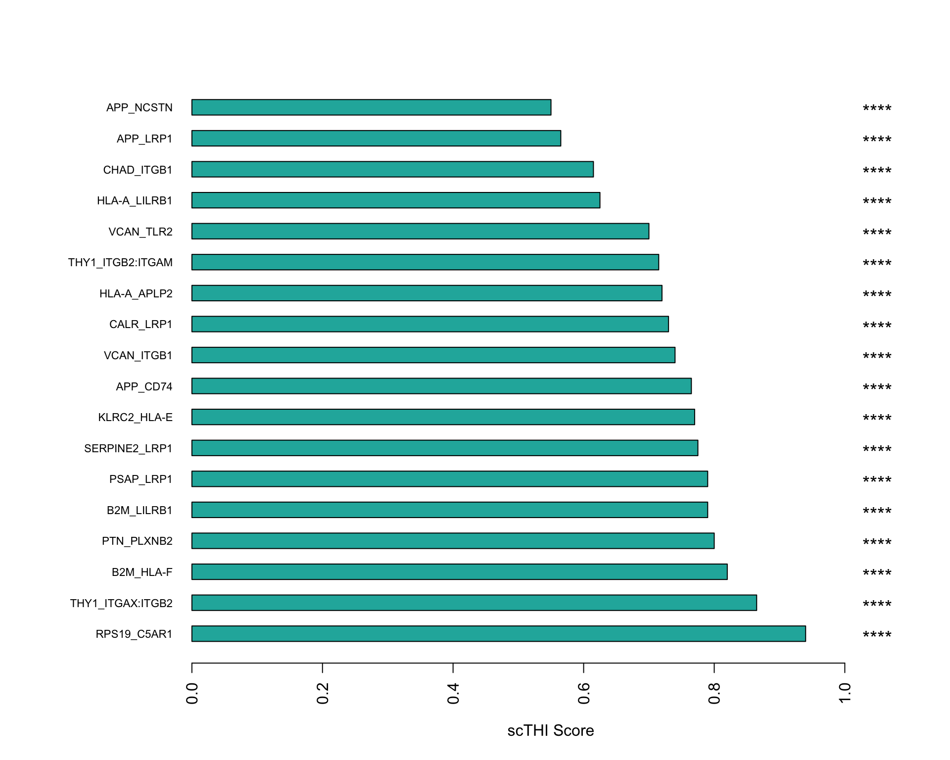
4.1 Scores
We can visualise a bar plot of the scores for the significant pairs.
scTHI_plotResult(
    scTHIresult = output,
    cexNames    = 0.7,
    plotType    = "score"
)
| Version | Author | Date |
|---|---|---|
| 38ee322 | Luke Zappia | 2020-11-10 |
Chunk time: 0.15 secs
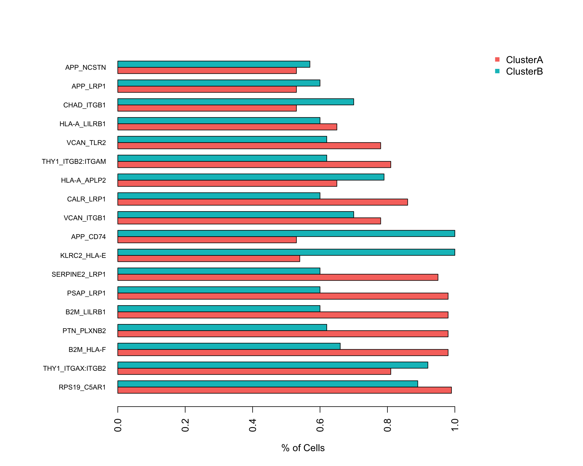
4.2 Expression
This bar plot shows the percentage of cells in each cluster that express each partner in the interaction.
scTHI_plotResult(
    scTHIresult = output,
    cexNames    = 0.7,
    plotType    = "pair"
)
| Version | Author | Date |
|---|---|---|
| 38ee322 | Luke Zappia | 2020-11-10 |
Chunk time: 0.1 secs
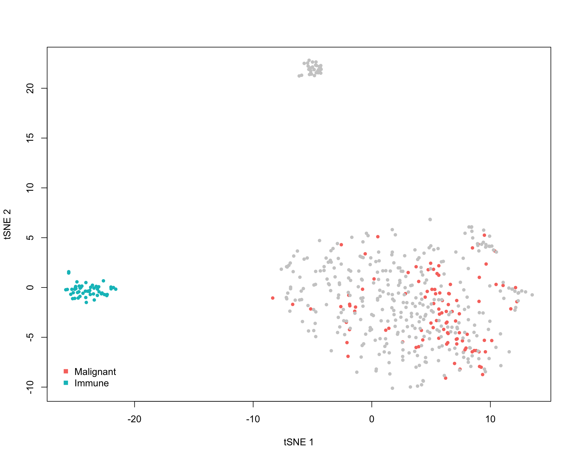
4.3 t-SNE
We can also look at where cells lie in a t-SNE embedding.
4.3.1 Cluster
Here the cells are coloured by the selected clusters.
output <- scTHI_runTsne(scTHIresult = output)

scTHI_plotCluster(
    scTHIresult = output,
    cexPoint    = 0.8,
    legendPos   = "bottomleft"
)
| Version | Author | Date |
|---|---|---|
| 38ee322 | Luke Zappia | 2020-11-10 |
Chunk time: 12.06 secs
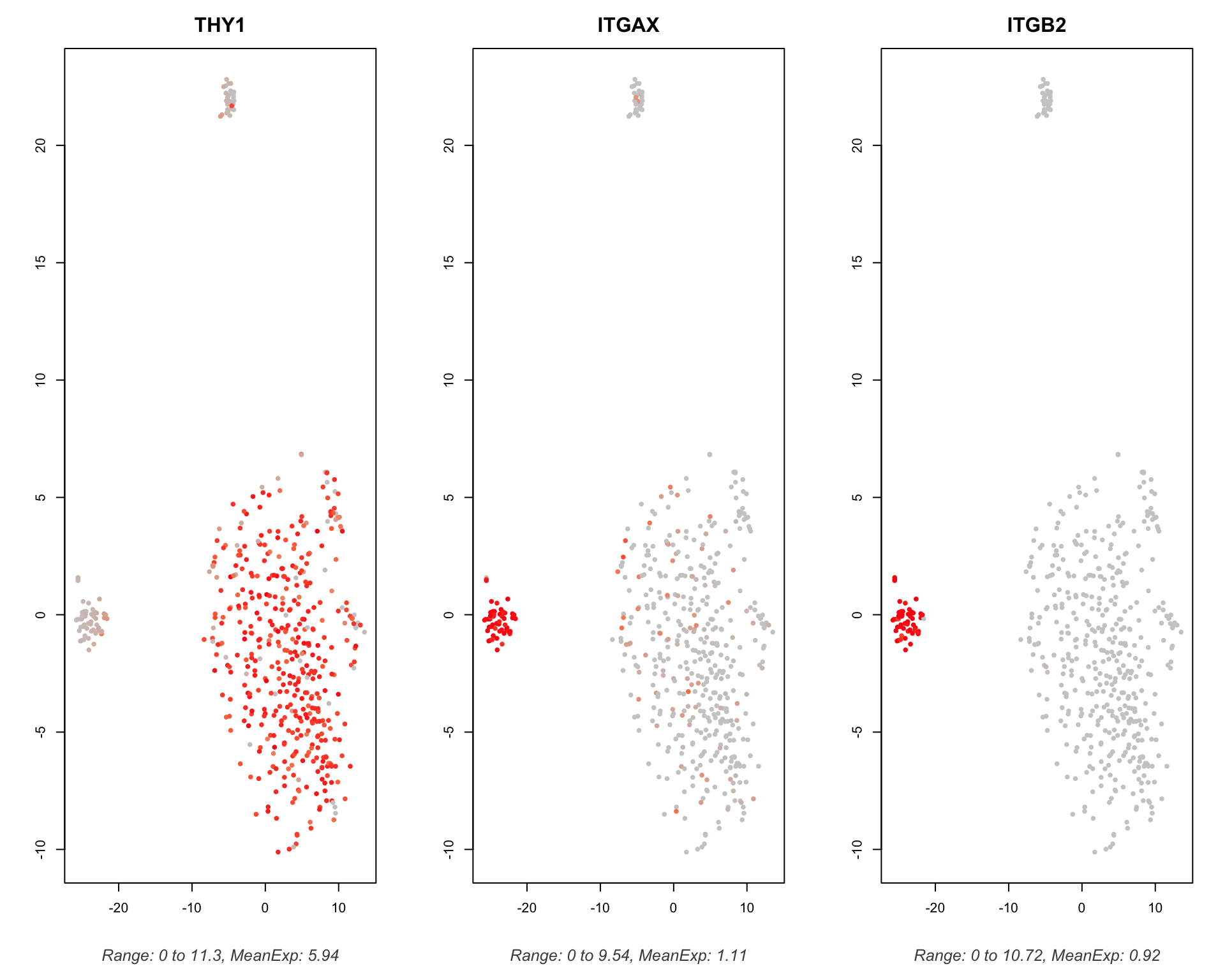
4.3.2 Interactions
We can also plot the expression of specific pairs we are interested in.
scTHI_plotPairs(
    scTHIresult       = output,
    cexPoint          = 0.8,
    interactionToplot = "THY1_ITGAX:ITGB2"
)
| Version | Author | Date |
|---|---|---|
| 38ee322 | Luke Zappia | 2020-11-10 |
Chunk time: 0.2 secs
Summary
Parameters
This table describes parameters used and set in this document.
params <- list(

)
params <- toJSON(params, pretty = TRUE)
kable(fromJSON(params))
Chunk time: 0.01 secs
Output files
This table describes the output files produced by this document. Right click and Save Link As… to download the results.
kable(data.frame(
    File = c(
        download_link("parameters.json", OUT_DIR)
    ),
    Description = c(
        "Parameters set and used in this analysis"
    )
))| File | Description |
|---|---|
| parameters.json | Parameters set and used in this analysis |
Chunk time: 0.01 secs
Session information
sessioninfo::session_info()─ Session info ───────────────────────────────────────────────────────────────
setting value
version R version 4.0.0 (2020-04-24)
os macOS Catalina 10.15.7
system x86_64, darwin17.0
ui X11
language (EN)
collate en_US.UTF-8
ctype en_US.UTF-8
tz Europe/Berlin
date 2020-11-24
─ Packages ───────────────────────────────────────────────────────────────────
! package * version date lib source
P assertthat 0.2.1 2019-03-21 [?] CRAN (R 4.0.0)
P backports 1.1.6 2020-04-05 [?] CRAN (R 4.0.0)
P base64enc 0.1-3 2015-07-28 [?] CRAN (R 4.0.0)
P base64url 1.4 2018-05-14 [?] standard (@1.4)
P BiocParallel 1.22.0 2020-04-27 [?] Bioconductor
P broom 0.5.6 2020-04-20 [?] CRAN (R 4.0.0)
P cellranger 1.1.0 2016-07-27 [?] standard (@1.1.0)
P cli 2.0.2 2020-02-28 [?] CRAN (R 4.0.0)
P colorspace 1.4-1 2019-03-18 [?] standard (@1.4-1)
P conflicted * 1.0.4 2019-06-21 [?] standard (@1.0.4)
P crayon 1.3.4 2017-09-16 [?] CRAN (R 4.0.0)
P DBI 1.1.0 2019-12-15 [?] CRAN (R 4.0.0)
P dbplyr 1.4.3 2020-04-19 [?] CRAN (R 4.0.0)
P digest 0.6.25 2020-02-23 [?] CRAN (R 4.0.0)
P dplyr * 0.8.5 2020-03-07 [?] CRAN (R 4.0.0)
P drake 7.12.0 2020-03-25 [?] CRAN (R 4.0.0)
P ellipsis 0.3.0 2019-09-20 [?] CRAN (R 4.0.0)
P evaluate 0.14 2019-05-28 [?] standard (@0.14)
P fansi 0.4.1 2020-01-08 [?] CRAN (R 4.0.0)
P filelock 1.0.2 2018-10-05 [?] CRAN (R 4.0.0)
P forcats * 0.5.0 2020-03-01 [?] CRAN (R 4.0.0)
P fs * 1.4.1 2020-04-04 [?] CRAN (R 4.0.0)
P generics 0.0.2 2018-11-29 [?] standard (@0.0.2)
P ggplot2 * 3.3.0 2020-03-05 [?] CRAN (R 4.0.0)
P git2r 0.27.1 2020-05-03 [?] CRAN (R 4.0.0)
P glue * 1.4.0 2020-04-03 [?] CRAN (R 4.0.0)
P gtable 0.3.0 2019-03-25 [?] standard (@0.3.0)
P haven 2.2.0 2019-11-08 [?] standard (@2.2.0)
P here * 0.1 2017-05-28 [?] standard (@0.1)
P highr 0.8 2019-03-20 [?] standard (@0.8)
P hms 0.5.3 2020-01-08 [?] CRAN (R 4.0.0)
P htmltools 0.5.0 2020-06-16 [?] CRAN (R 4.0.2)
P httpuv 1.5.2 2019-09-11 [?] standard (@1.5.2)
P httr 1.4.1 2019-08-05 [?] standard (@1.4.1)
P igraph 1.2.5 2020-03-19 [?] CRAN (R 4.0.0)
P jsonlite * 1.6.1 2020-02-02 [?] CRAN (R 4.0.0)
P knitr * 1.28 2020-02-06 [?] CRAN (R 4.0.0)
P later 1.0.0 2019-10-04 [?] standard (@1.0.0)
P lattice 0.20-41 2020-04-02 [?] CRAN (R 4.0.0)
P lifecycle 0.2.0 2020-03-06 [?] CRAN (R 4.0.0)
P lubridate 1.7.8 2020-04-06 [?] CRAN (R 4.0.0)
P magrittr 1.5 2014-11-22 [?] CRAN (R 4.0.0)
P Matrix 1.2-18 2019-11-27 [?] standard (@1.2-18)
P memoise 1.1.0 2017-04-21 [?] standard (@1.1.0)
P modelr 0.1.7 2020-04-30 [?] CRAN (R 4.0.0)
P munsell 0.5.0 2018-06-12 [?] standard (@0.5.0)
P nlme 3.1-147 2020-04-13 [?] CRAN (R 4.0.0)
P pander * 0.6.3 2018-11-06 [?] CRAN (R 4.0.0)
P pillar 1.4.4 2020-05-05 [?] CRAN (R 4.0.0)
P pkgconfig 2.0.3 2019-09-22 [?] CRAN (R 4.0.0)
P prettyunits 1.1.1 2020-01-24 [?] CRAN (R 4.0.0)
P progress 1.2.2 2019-05-16 [?] CRAN (R 4.0.0)
P promises 1.1.0 2019-10-04 [?] standard (@1.1.0)
P purrr * 0.3.4 2020-04-17 [?] CRAN (R 4.0.0)
P R6 2.4.1 2019-11-12 [?] CRAN (R 4.0.0)
P Rcpp 1.0.4.6 2020-04-09 [?] CRAN (R 4.0.0)
P readr * 1.3.1 2018-12-21 [?] standard (@1.3.1)
P readxl 1.3.1 2019-03-13 [?] standard (@1.3.1)
P renv 0.12.0 2020-08-28 [?] CRAN (R 4.0.2)
P repr 1.1.0 2020-01-28 [?] CRAN (R 4.0.0)
P reprex 0.3.0 2019-05-16 [?] standard (@0.3.0)
P reticulate 1.16 2020-05-27 [?] CRAN (R 4.0.2)
P rlang 0.4.6 2020-05-02 [?] CRAN (R 4.0.0)
P rmarkdown 2.1 2020-01-20 [?] CRAN (R 4.0.0)
P rprojroot 1.3-2 2018-01-03 [?] CRAN (R 4.0.0)
P rstudioapi 0.11 2020-02-07 [?] CRAN (R 4.0.0)
Rtsne 0.15 2018-11-10 [1] CRAN (R 4.0.0)
P rvest 0.3.5 2019-11-08 [?] standard (@0.3.5)
P scales 1.1.0 2019-11-18 [?] standard (@1.1.0)
P scTHI * 1.0.0 2020-04-27 [?] Bioconductor
P sessioninfo 1.1.1 2018-11-05 [?] CRAN (R 4.0.0)
P skimr * 2.1.1 2020-04-16 [?] CRAN (R 4.0.0)
P storr 1.2.1 2018-10-18 [?] standard (@1.2.1)
P stringi 1.4.6 2020-02-17 [?] CRAN (R 4.0.0)
P stringr * 1.4.0 2019-02-10 [?] CRAN (R 4.0.0)
P tibble * 3.0.1 2020-04-20 [?] CRAN (R 4.0.0)
P tidyr * 1.0.3 2020-05-07 [?] CRAN (R 4.0.0)
P tidyselect 1.0.0 2020-01-27 [?] CRAN (R 4.0.0)
P tidyverse * 1.3.0 2019-11-21 [?] standard (@1.3.0)
P txtq 0.2.0 2019-10-15 [?] standard (@0.2.0)
P vctrs 0.2.4 2020-03-10 [?] CRAN (R 4.0.0)
P whisker 0.4 2019-08-28 [?] standard (@0.4)
P withr 2.2.0 2020-04-20 [?] CRAN (R 4.0.0)
P workflowr 1.6.2 2020-04-30 [?] CRAN (R 4.0.0)
P xfun 0.13 2020-04-13 [?] CRAN (R 4.0.0)
P xml2 1.3.2 2020-04-23 [?] CRAN (R 4.0.0)
P yaml 2.2.1 2020-02-01 [?] CRAN (R 4.0.0)
[1] /Users/luke.zappia/Documents/Projects/interaction-tools/renv/library/R-4.0/x86_64-apple-darwin17.0
[2] /private/var/folders/rj/60lhr791617422kqvh0r4vy40000gn/T/RtmpOqMPdA/renv-system-library
[3] /private/var/folders/rj/60lhr791617422kqvh0r4vy40000gn/T/RtmpqYMqtc/renv-system-library
[4] /private/var/folders/rj/60lhr791617422kqvh0r4vy40000gn/T/Rtmp7wtwHE/renv-system-library
P ── Loaded and on-disk path mismatch.Chunk time: 0.16 secs