Human hematopoiesis - data preprocessing

Here, we process a human hematopoiesis dataset to infer the underlying dynamics with CellRank in further analyses. This workflow includes the standard preprocessing steps of scRNA-seq data, and the inference of a pseudotime with Palantir.

The corresponding data can be downloaded from here and should be saved in data/bone_marrow/raw/adata.h5ad, i.e.,

mkdir -p ../../data/bone_marrow/raw/
wget https://figshare.com/ndownloader/files/53393684 -O ../../data/bone_marrow/raw/adata.h5ad

Library imports

import warnings

import pandas as pd

import matplotlib as mpl
import matplotlib.pyplot as plt
import mplscience

import anndata as ad
import palantir
import scanpy as sc
import scvelo as scv

from crp import DATA_DIR, FIG_DIR

General settings

warnings.filterwarnings(action="ignore", category=FutureWarning)

sc.settings.verbosity = 2
scv.settings.verbosity = 3

mpl.use("module://matplotlib_inline.backend_inline")
mpl.rcParams["backend"]

plt.rcParams["font.family"] = "sans-serif"
plt.rcParams["font.sans-serif"] = ["Arial"]

scv.settings.set_figure_params("scvelo", dpi_save=400, dpi=80, transparent=True, fontsize=20, color_map="viridis")

Constants

SAVE_FIGURES = False
if SAVE_FIGURES:
    (FIG_DIR / "pseudotimekernel").mkdir(parents=True, exist_ok=True)

FIGURE_FORMAT = "svg"

SAVE_RESULTS = False
if SAVE_RESULTS:
    (DATA_DIR / "bone_marrow" / "processed").mkdir(parents=True, exist_ok=True)

Data loading

adata = ad.io.read_h5ad(DATA_DIR / "bone_marrow" / "raw" / "adata.h5ad")
adata

AnnData object with n_obs × n_vars = 6881 × 12464
    obs: 'leiden', 'celltype'
    var: 'highly_variable'
    uns: 'celltype_colors'
    obsm: 'X_umap'

Data preprocessing

sc.pp.normalize_per_cell(adata)
sc.pp.log1p(adata)
sc.pp.highly_variable_genes(adata, n_top_genes=1500, subset=True)

normalizing by total count per cell
    finished (0:00:00): normalized adata.X and added
    'n_counts', counts per cell before normalization (adata.obs)
extracting highly variable genes
    finished (0:00:00)

sc.tl.pca(adata, n_comps=50)
sc.pp.neighbors(adata, n_pcs=50, n_neighbors=30)

computing PCA
    with n_comps=50
    finished (0:00:00)
computing neighbors
    using 'X_pca' with n_pcs = 50
    finished (0:00:02)

sc.tl.umap(adata)

computing UMAP
    finished (0:00:05)

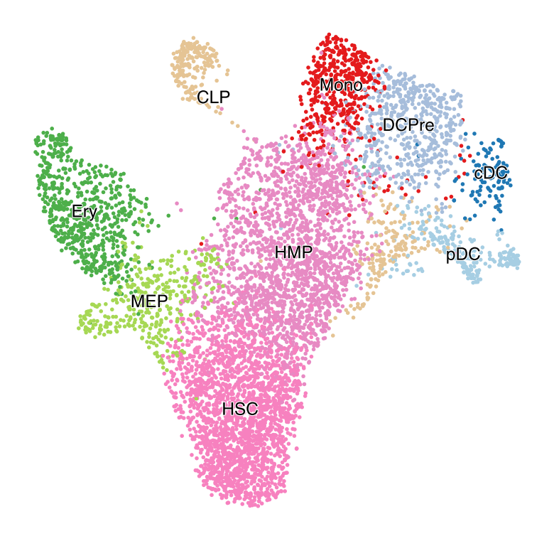
with mplscience.style_context():
    fig, ax = plt.subplots(figsize=(6, 6))
    scv.pl.scatter(adata, basis="umap", color=["celltype"], size=25, dpi=100, title="", ax=ax)
    plt.show()

if SAVE_FIGURES:
    fig, ax = plt.subplots(figsize=(6, 6))
    scv.pl.scatter(adata, basis="umap", color=["celltype"], size=25, dpi=100, title="", legend_loc=False, ax=ax)
    fig.savefig(
        FIG_DIR / "pseudotimekernel" / "umap_colored_by_cell_type.png",
        dpi=400,
        transparent=True,
        bbox_inches="tight",
    )

pc_projection = pd.DataFrame(adata.obsm["X_pca"].copy(), index=adata.obs_names)

# diffusion maps
diff_maps = palantir.utils.run_diffusion_maps(pc_projection, n_components=15)

computing neighbors
    finished (0:00:00)

adata.obsm["X_diffmap"] = diff_maps["EigenVectors"].values.copy()
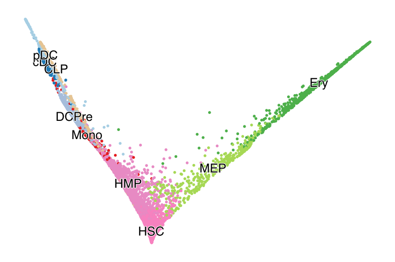
with mplscience.style_context():
    fig, ax = plt.subplots(figsize=(6, 4))
    scv.pl.scatter(adata, basis="diffmap", color=["celltype"], components=["1, 2"], size=25, dpi=100, title="", ax=ax)
    plt.show()

# multiscale space
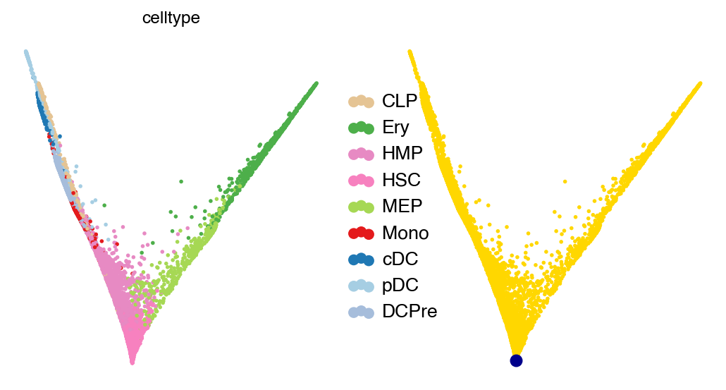
multiscale_space = palantir.utils.determine_multiscale_space(diff_maps)

root_idx = 3290  # adata.obsm["X_diffmap"][:, 2].argmin()
with mplscience.style_context():
    scv.pl.scatter(adata, basis="diffmap", color=["celltype", root_idx], legend_loc="right", components="1, 2", size=25)
    plt.show()

palantir_res = palantir.core.run_palantir(
    multiscale_space, adata.obs_names[root_idx], use_early_cell_as_start=True, num_waypoints=500
)

Sampling and flocking waypoints...
Time for determining waypoints: 0.000851603349049886 minutes
Determining pseudotime...
Shortest path distances using 30-nearest neighbor graph...
Time for shortest paths: 0.06112736860911051 minutes
Iteratively refining the pseudotime...
Correlation at iteration 1: 0.9996
Correlation at iteration 2: 1.0000
Entropy and branch probabilities...
Markov chain construction...
Identification of terminal states...
Computing fundamental matrix and absorption probabilities...
Project results to all cells...

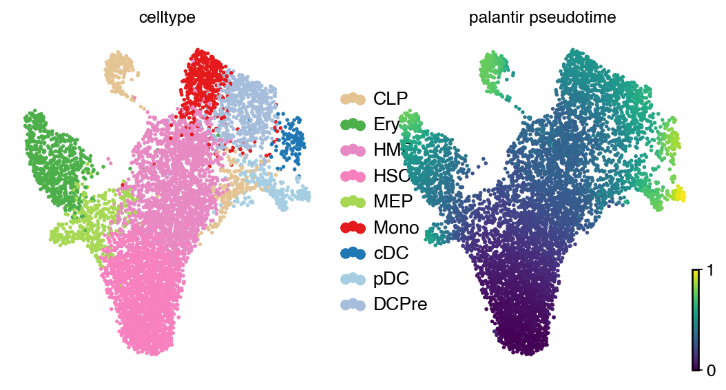
adata.obs["palantir_pseudotime"] = palantir_res.pseudotime

with mplscience.style_context():
    scv.pl.scatter(
        adata, basis="umap", color=["celltype", "palantir_pseudotime"], legend_loc="right", color_map="viridis", size=25
    )
    plt.show()

if SAVE_RESULTS:
    adata.write_h5ad(DATA_DIR / "bone_marrow" / "processed" / "adata.h5ad")