Heart alignment#
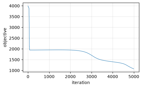
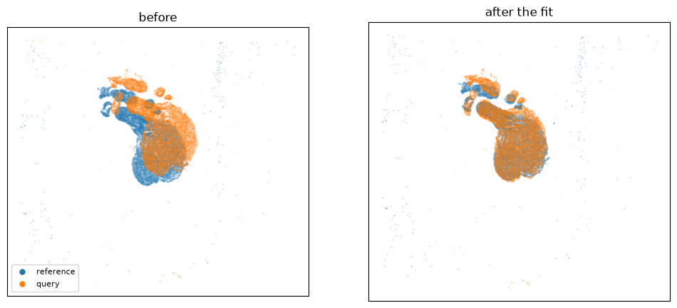
Two serial sections of the same heart. The tissue is far less regular than brain, so the matching term does most of the work and sigmaB is dropped to 0.1 to keep background from being read as tissue. Upstream caps this one at niter=1000, which is not enough: the two sections start 1742 um apart and at the default translation step that budget only closes it to 1587. Leaving niter alone – squidpy’s default is 5000, and so is upstream’s LDDMM’s – gets it to 238 um. Nothing else needed tuning; it was an iteration budget, not a parameter.
Upstream’s equivalent is heart-alignment. One call does the alignment: stalign_align_obs fits a
diffeomorphism straight between two point clouds, rasterizing both sides itself.
STalign’s own version of this analysis: heart-alignment.
Inputs#
import anndata as ad, numpy as np, pandas as pd

def read_xy(path, x, y, *, skip_first=False):
    df = pd.read_csv(path)
    xy = np.c_[np.asarray(df[x])[1:] if skip_first else df[x],
               np.asarray(df[y])[1:] if skip_first else df[y]].astype(float)
    return ad.AnnData(X=np.zeros((len(xy), 1)), obsm={'spatial': xy})

ref = read_xy('heart_data/CN73_E2.csv.gz', 'x', 'y')
query = read_xy('heart_data/CN73_E1.csv.gz', 'x', 'y')
print(f'{ref.n_obs} reference cells, {query.n_obs} query cells')
11771 reference cells, 12183 query cells
The fit#
Upstream’s own solver values, and squidpy’s defaults for everything else.
from squidpy.experimental.tl import stalign_align_obs

fit = stalign_align_obs(
    ref, query, spatial_key='spatial',
    dx=100.0, blur=1.0, epV=1000, sigmaB=0.1,
)
print(f'{fit.n_iter} iterations, objective '
      f'{float(fit.energies[0]):.0f} -> {float(fit.energies[-1]):.0f}')
5000 iterations, objective 3992 -> 1073
Where the cells land#
StalignFit.transform writes the mapped coordinates straight back into the query’s obsm,
so the alignment ends up on the object rather than in a local variable. It evaluates the fitted
map at each point, so a cell lands where it lands rather than at the nearest raster cell.
import matplotlib.pyplot as plt
from matplotlib.lines import Line2D
from scipy.spatial import cKDTree

fit.transform(query, key_added='aligned')
moved = query.obsm['aligned']

# Whether the fit worked, in the units of the data rather than of the objective. The energy
# can halve while the sections stay as far apart as they started -- that is what an iteration
# budget that ran out looks like, and it is invisible in the energy alone.
tree = cKDTree(ref.obsm['spatial'])
before = tree.query(query.obsm['spatial'])[0]
after = tree.query(moved)[0]
print(f"centroid offset {np.linalg.norm(query.obsm['spatial'].mean(0) - ref.obsm['spatial'].mean(0)):.0f}"
      f" -> {np.linalg.norm(moved.mean(0) - ref.obsm['spatial'].mean(0)):.0f}")
print(f'distance to the nearest reference cell: median {np.median(before):.0f} -> '
      f'{np.median(after):.0f}, 90th percentile {np.percentile(before, 90):.0f} -> '
      f'{np.percentile(after, 90):.0f}')

fig, ax = plt.subplots(1, 2, figsize=(12, 5.5))
for a, (pts, title) in zip(ax, [(query.obsm['spatial'], 'before'),
                                (moved, 'after the fit')], strict=True):
    a.scatter(*ref.obsm['spatial'].T, s=0.12, alpha=0.3, label='reference')
    a.scatter(*pts.T, s=0.12, alpha=0.3, label='query')
    a.set_title(title); a.set_aspect('equal'); a.invert_yaxis()
    a.set_xticks([]); a.set_yticks([])
ax[0].legend(handles=[Line2D([], [], marker='o', ls='', ms=5, color=c, label=l)
                     for c, l in (('tab:blue', 'reference'), ('tab:orange', 'query'))],
             loc='lower left', fontsize=8)
centroid offset 1742 -> 238
distance to the nearest reference cell: median 55 -> 33, 90th percentile 1031 -> 178
<matplotlib.legend.Legend at 0x7fa6799c9be0>
Convergence#
energies = np.asarray(fit.energies)[: fit.n_iter]
plt.figure(figsize=(5, 3))
plt.plot(energies, lw=0.8)
plt.xlabel('iteration'); plt.ylabel('objective'); plt.grid(alpha=0.3)