Placing MERFISH cells on a Visium H&E image#
When one side is an image there is nothing to rasterize it into, so the other side is
rasterized instead and stalign_align_image fits image to image.
The two live in different units – microns for the MERFISH section, pixels for the H&E – and
neither is restated anywhere: each element carries its own placement and the solver reads the
units off it. Upstream’s equivalent is merfish-visium-alignment.
STalign’s own version of this analysis: merfish-visium-alignment.
Inputs#
import matplotlib.pyplot as plt
import numpy as np, pandas as pd, spatialdata as sd
from spatialdata.models import Image2DModel, PointsModel
from spatialdata.transformations import get_transformation
from squidpy.experimental.im import rasterize_points

MERFISH = ('merfish_data/datasets_mouse_brain_map_BrainReceptorShowcase'
           '_Slice2_Replicate3_cell_metadata_S2R3.csv.gz')
cells = pd.read_csv(MERFISH)
xy = np.c_[cells['center_x'], cells['center_y']].astype(float)

# Both sides onto [0, 1], as upstream does: the solver's sigmas are in these units, and a raw
# density raster spans nothing like the range an image does.
def unit(a):
    a = np.asarray(a, dtype=float)
    return (a - a.min()) / np.ptp(a)

he = plt.imread('visium_data/tissue_hires_image.png')[..., :3]
visium = sd.SpatialData(images={'he': Image2DModel.parse(
    unit(np.moveaxis(he, -1, 0)), dims=('c', 'y', 'x'))})

merfish = sd.SpatialData(points={'cells': PointsModel.parse(xy)})
rasterize_points(merfish, points_key='cells', dx=30.0, blur=1.0, key_added='section')
element = merfish.images['section']
merfish.images['section'] = Image2DModel.parse(
    unit(np.asarray(element)), dims=('c', 'y', 'x'),
    transformations={'global': get_transformation(element, 'global')})
print(f'{len(xy)} cells rasterized to {tuple(np.asarray(merfish["section"]).shape)}, '
      f'H&E is {he.shape}')
85958 cells rasterized to (1, 256, 336), H&E is (2000, 1838, 3)
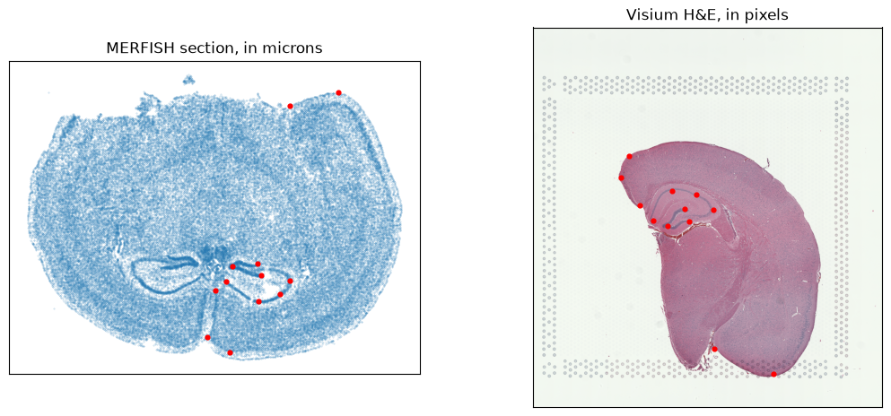
Twelve landmark pairs, matched by row order, each side in its own units – microns for the section, pixels for the H&E. Neither is restated anywhere: the elements carry their placement and the solver reads the units off them.
# Upstream's own pairs for this notebook, twelve of them, stored as `(x, y)` -- which is what
# squidpy takes, so nothing is transposed on the way in. The region-keyed `.npy` files belong to
# the point-annotator variant rather than to this one.
data = np.load('visium_data/visium2_points.npz')
paired = {'query': np.asarray(data['pointsI'], dtype=float),
          'ref': np.asarray(data['pointsJ'], dtype=float)}
print(f'{len(paired["ref"])} landmark pairs')

fig, ax = plt.subplots(1, 2, figsize=(13, 5.5))
ax[0].scatter(*xy.T, s=0.12, alpha=0.3); ax[0].scatter(*paired['query'].T, s=12, c='red')
ax[0].set_title('MERFISH section, in microns'); ax[0].invert_yaxis(); ax[0].set_aspect('equal')
ax[1].imshow(he); ax[1].scatter(*paired['ref'].T, s=12, c='red')
ax[1].set_title('Visium H&E, in pixels')
for a in ax:
    a.set_xticks([]); a.set_yticks([])
12 landmark pairs
The fit#
Upstream’s own solver values for this pair. sigmaP weights the landmark matching term, which
matters more here than in the point-cloud case: the two modalities do not share an intensity
scale, so the landmarks carry much of the correspondence.
from squidpy.experimental.tl import stalign_align_image

fit = stalign_align_image(
    visium, merfish, image_key=('he', 'section'),
    landmarks_ref=paired['ref'], landmarks_query=paired['query'],
    niter=200, sigmaM=0.2, sigmaB=0.19, sigmaA=0.3, sigmaP=2e-1,
    epL=5e-11, epT=5e-4, epV=5e1,
)
print(f'{fit.n_iter} iterations, objective '
      f'{float(fit.energies[0]):.0f} -> {float(fit.energies[-1]):.0f}')
200 iterations, objective 2055284 -> 555064
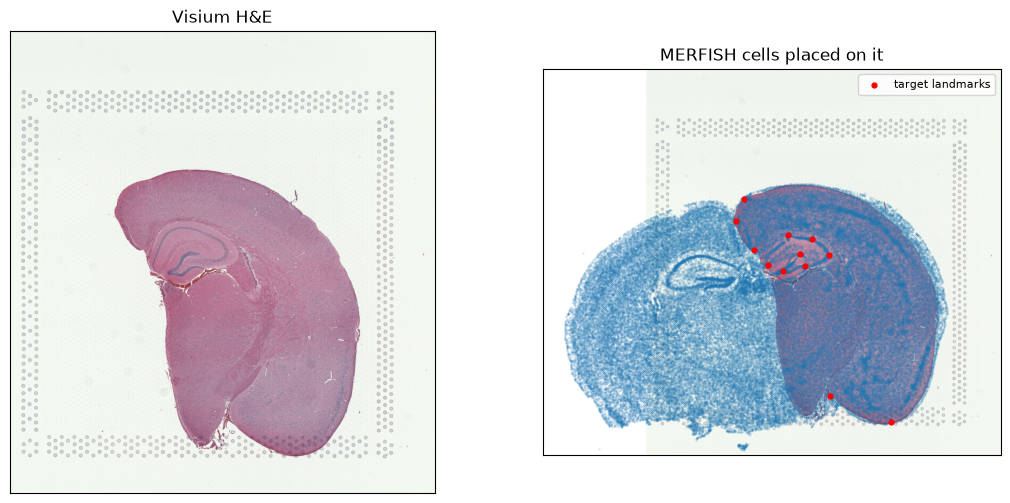
Every cell, placed on the image#
The H&E covers one hemisphere; the MERFISH section is a whole coronal slice. So roughly half the cells have no tissue to land on and end up beside the image rather than on it. That is the data, not a failed fit – upstream’s own notebook pairs these same two files and its published figure shows the same overhang.
It is also why the landmark residual below is not evidence of much: all twelve landmarks sit on the covered hemisphere, so the fit can satisfy them exactly while the uncovered half is pulled along by the deformation alone, with nothing to match against. The fraction of cells landing inside the image is the number that actually describes the situation.
placed = np.asarray(fit.transform_points(xy))
moved_landmarks = np.asarray(fit.transform_points(paired['query']))
residual = np.linalg.norm(moved_landmarks - paired['ref'], axis=1)
print(f'landmark residual after fitting: median {np.median(residual):.1f} px, '
      f'worst {residual.max():.1f} px')

rows, columns = he.shape[:2]
inside = ((placed[:, 0] >= 0) & (placed[:, 0] < columns)
          & (placed[:, 1] >= 0) & (placed[:, 1] < rows))
print(f'{inside.sum()} of {len(placed)} cells ({100 * inside.mean():.0f}%) land within the '
      f'{columns} x {rows} image; the rest are the hemisphere it does not cover')

fig, ax = plt.subplots(1, 2, figsize=(13, 6))
ax[0].imshow(he); ax[0].set_title('Visium H&E')
ax[1].imshow(he)
ax[1].scatter(*placed.T, s=0.12, alpha=0.3, c='tab:blue')
ax[1].scatter(*paired['ref'].T, s=12, c='red', label='target landmarks')
ax[1].set_title('MERFISH cells placed on it'); ax[1].legend(fontsize=8)
for a in ax:
    a.set_xticks([]); a.set_yticks([])
landmark residual after fitting: median 0.8 px, worst 5.1 px
72014 of 85958 cells (84%) land within the 1838 x 2000 image; the rest are the hemisphere it does not cover