Xenium xenium#
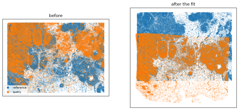
Two Xenium replicates of the same breast-cancer block. They overlap only partially, so some cells have no counterpart at all – the matching weights are what identify the supported overlap, and unmatched cells are expected rather than a failure.
Upstream’s equivalent is xenium-xenium-alignment. One call does the alignment: stalign_align_obs fits a
diffeomorphism straight between two point clouds, rasterizing both sides itself.
STalign’s own version of this analysis: xenium-xenium-alignment.
Inputs#
import anndata as ad, numpy as np, pandas as pd

def read_xy(path, x, y, *, skip_first=False):
    df = pd.read_csv(path)
    xy = np.c_[np.asarray(df[x])[1:] if skip_first else df[x],
               np.asarray(df[y])[1:] if skip_first else df[y]].astype(float)
    return ad.AnnData(X=np.zeros((len(xy), 1)), obsm={'spatial': xy})

ref = read_xy('xenium_data/Xenium_FFPE_Human_Breast_Cancer_Rep1_cells.csv.gz', 'x_centroid', 'y_centroid')
query = read_xy('xenium_data/Xenium_FFPE_Human_Breast_Cancer_Rep2_cells.csv.gz', 'x_centroid', 'y_centroid')

# Landmark pairs picked by hand, one array per side, matched by row order.
def read_landmarks(path):
    picked = np.load(path, allow_pickle=True).item()
    return np.array([p for key in sorted(picked) for p in picked[key]], dtype=float)

landmarks_ref = read_landmarks('xenium_data/Xenium_Breast_Cancer_Rep1_points.npy')
landmarks_query = read_landmarks('xenium_data/Xenium_Breast_Cancer_Rep2_points.npy')
print(f'{ref.n_obs} reference cells, {query.n_obs} query cells, '
      f'{len(landmarks_ref)} landmark pairs')
167782 reference cells, 118752 query cells, 3 landmark pairs
The fit#
Upstream’s own solver values, and squidpy’s defaults for everything else.
from squidpy.experimental.tl import stalign_align_obs

fit = stalign_align_obs(
    ref, query, spatial_key='spatial',
    landmarks_ref=landmarks_ref, landmarks_query=landmarks_query,
    dx=30.0, blur=1.0, niter=300, epV=100, sigmaM=1.5, sigmaB=1.0, sigmaA=1.1,
)
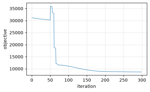
print(f'{fit.n_iter} iterations, objective '
      f'{float(fit.energies[0]):.0f} -> {float(fit.energies[-1]):.0f}')
300 iterations, objective 31182 -> 8661
Where the cells land#
StalignFit.transform writes the mapped coordinates straight back into the query’s obsm,
so the alignment ends up on the object rather than in a local variable. It evaluates the fitted
map at each point, so a cell lands where it lands rather than at the nearest raster cell.
import matplotlib.pyplot as plt
from matplotlib.lines import Line2D
from scipy.spatial import cKDTree

fit.transform(query, key_added='aligned')
moved = query.obsm['aligned']

# Whether the fit worked, in the units of the data rather than of the objective. The energy
# can halve while the sections stay as far apart as they started -- that is what an iteration
# budget that ran out looks like, and it is invisible in the energy alone.
tree = cKDTree(ref.obsm['spatial'])
before = tree.query(query.obsm['spatial'])[0]
after = tree.query(moved)[0]
print(f"centroid offset {np.linalg.norm(query.obsm['spatial'].mean(0) - ref.obsm['spatial'].mean(0)):.0f}"
      f" -> {np.linalg.norm(moved.mean(0) - ref.obsm['spatial'].mean(0)):.0f}")
print(f'distance to the nearest reference cell: median {np.median(before):.0f} -> '
      f'{np.median(after):.0f}, 90th percentile {np.percentile(before, 90):.0f} -> '
      f'{np.percentile(after, 90):.0f}')

fig, ax = plt.subplots(1, 2, figsize=(12, 5.5))
for a, (pts, title) in zip(ax, [(query.obsm['spatial'], 'before'),
                                (moved, 'after the fit')], strict=True):
    a.scatter(*ref.obsm['spatial'].T, s=0.12, alpha=0.3, label='reference')
    a.scatter(*pts.T, s=0.12, alpha=0.3, label='query')
    a.set_title(title); a.set_aspect('equal'); a.invert_yaxis()
    a.set_xticks([]); a.set_yticks([])
ax[0].legend(handles=[Line2D([], [], marker='o', ls='', ms=5, color=c, label=l)
                     for c, l in (('tab:blue', 'reference'), ('tab:orange', 'query'))],
             loc='lower left', fontsize=8)
centroid offset 625 -> 1249
distance to the nearest reference cell: median 6 -> 6, 90th percentile 22 -> 22
<matplotlib.legend.Legend at 0x7f9090181d30>
Convergence#
energies = np.asarray(fit.energies)[: fit.n_iter]
plt.figure(figsize=(5, 3))
plt.plot(energies, lw=0.8)
plt.xlabel('iteration'); plt.ylabel('objective'); plt.grid(alpha=0.3)