Aligning Xenium cells with their H&E image#
stalign_align_image fits image to image, so the cell cloud is rasterized first and the H&E is
matched against that raster. Upstream’s equivalent is xenium-heimage-alignment.
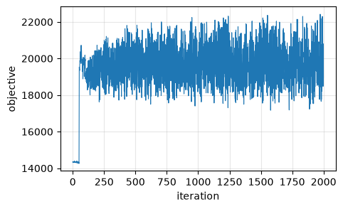
Which side is the reference matters here, and it is not a presentation choice. The objective is computed on the reference’s grid. Make the H&E the reference and it is evaluated over 2051 x 2759 x 3 pixels against a 201 x 276 section – roughly three hundred times more reference pixels than there is section to match – and the deformation gets driven by H&E texture with no counterpart: measured, the landmarks start 16 px apart and the fit walks them out to 524. With the raster as the reference the same fit starts at an objective of 14,352 instead of 4,417,134 and ends better than it started. So the rasterized cells are the reference, as upstream has it.
STalign’s own version of this analysis: xenium-heimage-alignment.
Inputs#
import matplotlib.pyplot as plt
import numpy as np, pandas as pd, spatialdata as sd
from spatialdata.models import Image2DModel, PointsModel
from spatialdata.transformations import get_transformation
from squidpy.experimental.im import rasterize_points
from squidpy.experimental.tl import stalign_align_image

# `sigmaM`, `sigmaB` and `sigmaA` are in the images' own intensity units, and upstream states
# its values for both sides mapped onto [0, 1]. A raw density raster of 167k cells has a mean
# near 3 and a max well above 10, which leaves widths of ~0.1 about a hundred times too tight:
# the fit then converges on an objective that has stopped measuring the overlap.
def unit(a):
    a = np.asarray(a, dtype=float)
    return (a - a.min()) / np.ptp(a)

def as_image(rgb, key):
    return sd.SpatialData(images={key: Image2DModel.parse(
        unit(np.moveaxis(rgb, -1, 0)), dims=('c', 'y', 'x'))})

def rasterized(xy, dx):
    sdata = sd.SpatialData(points={'cells': PointsModel.parse(xy)})
    rasterize_points(sdata, points_key='cells', dx=dx, blur=1.0, key_added='section')
    element = sdata.images['section']
    sdata.images['section'] = Image2DModel.parse(
        unit(np.asarray(element)), dims=('c', 'y', 'x'),
        transformations={'global': get_transformation(element, 'global')})
    return sdata

he = plt.imread('xenium_data/Xenium_FFPE_Human_Breast_Cancer_Rep1_he_image.png')[..., :3]
cells = pd.read_csv('xenium_data/Xenium_FFPE_Human_Breast_Cancer_Rep1_cells.csv.gz')
xy = np.c_[cells['x_centroid'], cells['y_centroid']].astype(float)

image = as_image(he, 'he')
section = rasterized(xy, 30.0)
print(f'{len(xy)} cells over {xy[:, 0].max():.0f} x {xy[:, 1].max():.0f} um, '
      f'rasterized to {tuple(np.asarray(section["section"]).shape)}; H&E is {he.shape}')
167782 cells over 7523 x 5476 um, rasterized to (1, 201, 276); H&E is (2051, 2759, 3)
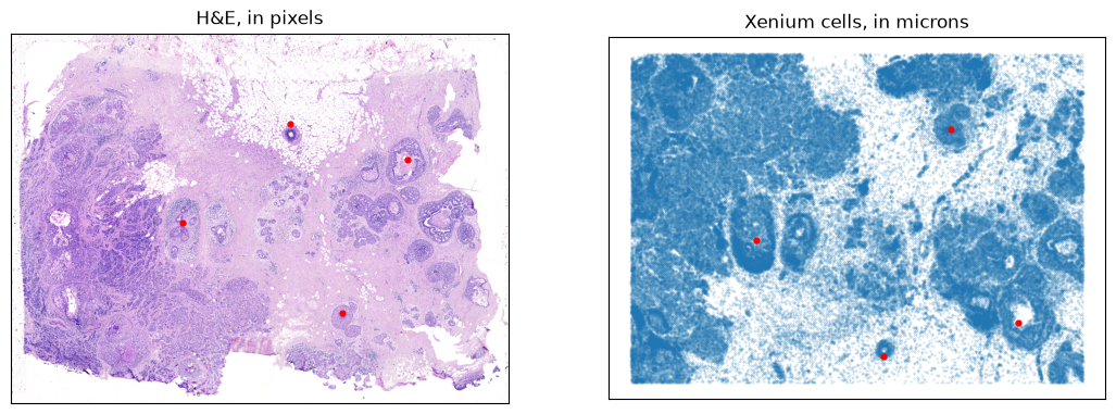
Four landmark pairs, hardcoded upstream. They are stored there as (y, x); squidpy’s public API
takes (x, y), so each is reversed once on the way in. Only one reading is even possible –
read as (x, y), the second H&E point’s 2200 would exceed the image’s 2051 height.
landmarks_he = np.array([[1050., 950.], [700., 2200.], [500., 1550.], [1550., 1840.]])[:, ::-1]
landmarks_cells = np.array([[3108., 2100.], [4480., 6440.], [5040., 4200.], [1260., 5320.]])[:, ::-1]

fig, ax = plt.subplots(1, 2, figsize=(13, 5.5))
ax[0].imshow(he); ax[0].scatter(*landmarks_he.T, s=12, c='red')
ax[0].set_title('H&E, in pixels')
ax[1].scatter(*xy.T, s=0.12, alpha=0.3); ax[1].scatter(*landmarks_cells.T, s=12, c='red')
ax[1].set_title('Xenium cells, in microns'); ax[1].invert_yaxis(); ax[1].set_aspect('equal')
for a in ax:
    a.set_xticks([]); a.set_yticks([])
The fit#
Upstream’s own solver values.
fit = stalign_align_image(
    section, image, image_key=('section', 'he'),
    landmarks_ref=landmarks_cells, landmarks_query=landmarks_he,
    niter=2000, sigmaM=0.15, sigmaB=0.10, sigmaA=0.11, epV=10,
)
print(f'{fit.n_iter} iterations, objective '
      f'{float(fit.energies[0]):.0f} -> {float(fit.energies[-1]):.0f}')

residual = np.linalg.norm(np.asarray(fit.transform_points(landmarks_he)) - landmarks_cells, axis=1)
print(f'landmark residual: median {np.median(residual):.1f} um, worst {residual.max():.1f} um')
2000 iterations, objective 14352 -> 18965
landmark residual: median 59.9 um, worst 75.9 um
The two together#
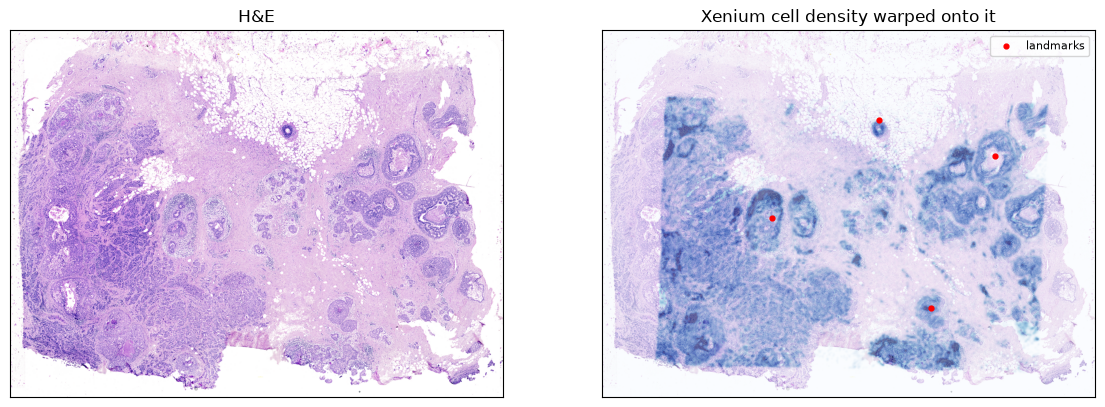
StalignFit.transform_points maps the query into the reference frame, which here is H&E pixels into microns –
the opposite of what a picture of cells-on-tissue wants. StalignImageFit.inverse_warp_image supplies the other
direction: it resamples a reference-frame image onto the query’s grid, so the cell density
lands on the H&E’s own pixels. That is the figure upstream publishes for this pair.
Going the other way for points – cells into H&E pixels – is
inverse_transform_points.
def physical_axes(element):
    matrix = get_transformation(element, 'global').to_affine_matrix(
        input_axes=('y', 'x'), output_axes=('y', 'x'))
    return tuple((np.asarray(element.coords[a]) - 0.5) * matrix[k, k] + matrix[k, -1]
                 for k, a in enumerate(('y', 'x')))

# The fit runs on upstream's dx=30 raster -- 201 x 276 -- and resampling that onto 2051 x 2759
# is a tenfold upsample, so it arrives soft no matter how it is drawn. `warp_image` takes
# explicit axes for exactly this: the same fitted deformation can carry a finer raster, which
# has the detail to survive the trip. The fit is unchanged; only what is pushed through it is.

display = rasterized(xy, 8.0)
density = np.asarray(fit.inverse_warp_image(np.asarray(display['section']),
    ref_axes=physical_axes(display['section']))).squeeze()
print(f'fitted on {tuple(np.asarray(section["section"]).shape)}, '
      f'displayed through a {tuple(np.asarray(display["section"]).shape)} raster '
      f'-> {density.shape}')

fig, ax = plt.subplots(1, 2, figsize=(14, 6))
ax[0].imshow(he); ax[0].set_title('H&E')
ax[1].imshow(he)
# Clipped at a high percentile rather than the max: a few dense cores otherwise take the whole
# colour range and flatten everything else to nothing.
ax[1].imshow(density, cmap='Blues', alpha=0.55, vmin=0,
             vmax=np.percentile(density[density > 0], 99))
ax[1].scatter(*landmarks_he.T, s=12, c='red', label='landmarks')
ax[1].set_title('Xenium cell density warped onto it'); ax[1].legend(fontsize=8)
for a in ax:
    a.set_xticks([]); a.set_yticks([])
fitted on (1, 201, 276), displayed through a (1, 753, 1035) raster -> (2051, 2759)
Convergence#
energies = np.asarray(fit.energies)[: fit.n_iter]
plt.figure(figsize=(5, 3))
plt.plot(energies, lw=0.8)
plt.xlabel('iteration'); plt.ylabel('objective'); plt.grid(alpha=0.3)