Placing a STARmap section in the Allen CCF#
A 2D section fitted into a 3D reference volume, entirely through squidpy’s public API:
rasterize_points -> stalign_align_volume -> StalignFit.transform_points -> sample_volume.
STalign’s own version of this analysis: starmap-allen3Datlas-alignment.
Inputs#
Cells as a points element, the atlas and its annotation volume as 3D images. The physical placement lives on the elements, so nothing downstream builds coordinate axes by hand.
import nrrd, numpy as np, pandas as pd, spatialdata as sd
from spatialdata.models import Image3DModel, PointsModel
from spatialdata.transformations import Scale, Sequence, Translation

cells = pd.read_csv('starmap_data/well11_spatial.csv.gz')
xy = np.c_[np.array(cells['X'])[1:], np.array(cells['Y'])[1:]].astype(float)

atlas, hdr = nrrd.read('ara_nissl_50.nrrd')       # (z, y, x)
labels, _ = nrrd.read('annotation_50.nrrd')       # same frame, integer structure ids
voxel = tuple(np.diag(hdr['space directions']))

def unit_range(a):
    return (a - a.min()) / np.ptp(a)

# The second channel is not decoration: the solver regresses the deformed reference onto the
# section before measuring the match, so one channel fits `a + b*I` and two fit
# `a + b*I + c*(I - mean I)**2`. A regression absorbs a rescaling of its input; it cannot
# invent a channel it was never handed.
def reference_channels(volume):
    v = volume[None] / np.mean(np.abs(volume))
    return np.concatenate([v, (v - v.mean()) ** 2])

sdata = sd.SpatialData(
    points={'cells': PointsModel.parse(xy)},
    images={'atlas': Image3DModel.parse(
        unit_range(reference_channels(atlas.astype(float))), dims=('c', 'z', 'y', 'x'),
        transformations={'global': Sequence([
            Scale(list(voxel), axes=('z', 'y', 'x')),
            Translation(-(np.asarray(atlas.shape) - 1) * np.asarray(voxel) / 2,
                        axes=('z', 'y', 'x')),
        ])},
    )},
)
sdata
SpatialData object
├── Images
│     └── 'atlas': DataArray[czyx] (2, 264, 160, 228)
└── Points
      └── 'cells': DataFrame with shape: (<Delayed>, 2) (2D points)
with coordinate systems:
    ▸ 'global', with elements:
        atlas (Images), cells (Points)
The section#
rasterize_points turns the centroids into a density image: each cell deposits unit mass
bilinearly, blurred once per scale, so total intensity is exactly the cell count.
from squidpy.experimental.im import rasterize_points, sample_volume

rasterize_points(sdata, points_key='cells', dx=50.0, blur=1.0, key_added='section')
sdata['section']
<xarray.DataArray 'image' (c: 1, y: 563, x: 760)> Size: 3MB
dask.array<array, shape=(1, 563, 760), dtype=float64, chunksize=(1, 563, 760), chunktype=numpy.ndarray>
Coordinates:
  * c        (c) int64 8B 0
  * y        (y) float64 5kB 0.5 1.5 2.5 3.5 4.5 ... 559.5 560.5 561.5 562.5
  * x        (x) float64 6kB 0.5 1.5 2.5 3.5 4.5 ... 756.5 757.5 758.5 759.5
Attributes:
transform: {'global': Sequence \n Scale (y, x)\n [50. 50.]\n ...Putting both volumes on the scale the solver’s parameters assume#
sigmaM, sigmaA, sigmaB, muA and muB are in the target’s intensity units, and
upstream states its values against a section that has been divided by its own mean and then
mapped onto [0, 1]. The reference gets the same treatment, which the solver’s intensity
regression would absorb on its own – but the second channel it is given alongside is not
something any regression can recover, so both steps are done here rather than assumed.
from spatialdata.models import Image2DModel
from spatialdata.transformations import get_transformation

def mean_normalised(sdata, key):
    element = sdata.images[key]
    values = np.asarray(element)
    sdata.images[key] = Image2DModel.parse(
        values / np.abs(values).mean(), dims=('c', 'y', 'x'),
        transformations={'global': get_transformation(element, 'global')},
    )

mean_normalised(sdata, 'section')
element = sdata.images['section']
sdata.images['section'] = Image2DModel.parse(
    unit_range(np.asarray(element)), dims=('c', 'y', 'x'),
    transformations={'global': get_transformation(element, 'global')},
)
section = np.asarray(sdata['section']).squeeze()
print(f'section now spans {section.min():.2f} to {section.max():.2f}, mean {section.mean():.2f}')
section now spans 0.00 to 1.00, mean 0.10
The fit#
The starting guess only has to be close. initial_affine places the section in the atlas –
an explicit matrix here rather than the initial_* arguments, because this dataset is
anisotropic and initial_scale is a single uniform factor – and the fit then deforms the
volume in all three dimensions rather than searching for a flat plane through it.
from squidpy.experimental.tl import stalign_align_volume

def physical_axes(element, axes):
    matrix = get_transformation(element, 'global').to_affine_matrix(input_axes=axes, output_axes=axes)
    return [(np.asarray(element.coords[a]) - 0.5) * matrix[k, k] + matrix[k, -1]
            for k, a in enumerate(axes)]

# `initial_scale` is one uniform factor for all three axes, and this dataset is anisotropic:
# ~4x in plane, ~0.9x through the slice axis. `initial_affine` is the escape hatch.
#
# Built in the solver's (z, y, x) and reversed once at the end. Composing it directly in
# (x, y, z) means hand-transposing a rotation, two scales and three translations, and each is
# a chance to mirror an axis silently -- so the reversal gets exactly one line.
theta, scale_xy, scale_z, slice_index = np.pi / 2, 4.0, 0.9, 140
z_axis, _, _ = physical_axes(sdata['atlas'], ('z', 'y', 'x'))
y_axis, x_axis = physical_axes(sdata['section'], ('y', 'x'))

# The one landmark this analysis pins: atlas (0, 0) sits at (-3700, 0) in the section, in (-y, -x).
landmark_yx = np.array([-3700.0, 0.0])

rotation = np.array([[1.0, 0.0, 0.0],
                     [0.0, np.cos(theta), -np.sin(theta)],
                     [0.0, np.sin(theta), np.cos(theta)]])
affine_zyx = np.eye(4)
affine_zyx[:3, :3] = rotation @ np.diag([scale_z, scale_xy, scale_xy])
affine_zyx[:3, 3] = [-z_axis[slice_index],
                     y_axis.mean() - landmark_yx[0] * scale_xy,
                     x_axis.mean() - landmark_yx[1] * scale_xy]

reverse = np.eye(4)[[2, 1, 0, 3]]          # spatial axes only; the homogeneous row stays put
initial_affine = np.linalg.inv(reverse @ affine_zyx @ reverse)  # section -> volume

# `sigmaR` is deliberately absent. Upstream's `LDDMM_3D_to_slice` declares 1e8, which weights
# the regulariser so weakly that the velocity field grows unchecked; squidpy's volume default
# is the retuned 1e6, and letting the default supply it is the point.
SOLVER = dict(a=250.0, nt=4, sigmaM=0.1, sigmaA=0.1, sigmaB=0.1, muA=[0.7], muB=[0.0])
fit = stalign_align_volume(
    sdata, image_key=('atlas', 'section'), initial_affine=initial_affine, niter=800, **SOLVER
)
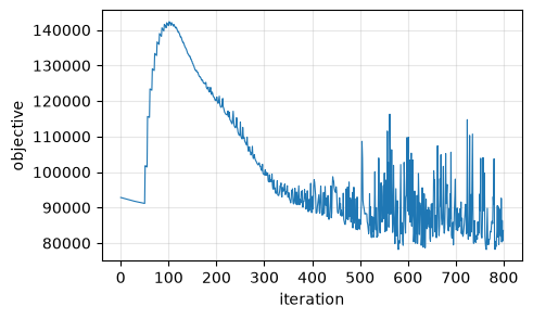
print(f'{fit.n_iter} iterations, objective '
      f'{float(fit.energies[0]):.0f} -> {float(fit.energies[-1]):.0f}')
800 iterations, objective 92837 -> 83538
Convergence#
import matplotlib.pyplot as plt

energies = np.asarray(fit.energies)[: fit.n_iter]
plt.figure(figsize=(5, 3))
plt.plot(energies, lw=0.8)
plt.xlabel('iteration'); plt.ylabel('objective'); plt.grid(alpha=0.3)
Where each cell lands#
StalignFit.transform_points maps (x, y) section coordinates to (x, y, z) reference coordinates, evaluated at
each point rather than at the nearest raster cell. sample_volume then reads the annotation
volume there – order=0 because structure ids must not be interpolated.
coords = np.asarray(fit.transform_points(xy))  # (N, 3), (x, y, z) in microns
structure_id = sample_volume(labels, coords, axes=fit.ref_axes, order=0).astype(int)

print(f'{len(coords)} cells placed, {np.unique(structure_id).size} distinct structures, '
      f'{100 * (structure_id == 0).mean():.1f}% outside any annotated structure')
print(f'depth (z) spans {coords[:, 2].min():.0f} to {coords[:, 2].max():.0f} um')
43341 cells placed, 168 distinct structures, 2.2% outside any annotated structure
depth (z) spans 468 to 812 um
Structure ids become acronyms through the Allen ontology.
ontology = pd.read_csv('allen_ontology.csv').set_index('id')['acronym']
acronym = pd.Series(structure_id).map(ontology).fillna('unassigned')
acronym.value_counts().head(12)
CP            1450
CA1           1450
MEA           1425
DG-sg         1243
PIR           1219
VPM           1202
or             993
unassigned     947
ccs            808
LHA            765
HY             705
PO             665
Name: count, dtype: int64
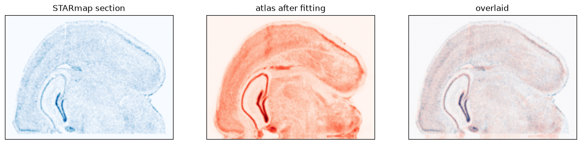
The aligned atlas over the section#
import matplotlib as mpl
from matplotlib.lines import Line2D

def atlas_at(result):
    plane = np.moveaxis(np.asarray(result.deformation_grid()), 0, -1)[0]
    sampled = sample_volume(atlas, plane.reshape(-1, 3)[:, ::-1], axes=result.ref_axes)
    return sampled.reshape(plane.shape[:2])

section = np.asarray(sdata['section']).squeeze()
fig, ax = plt.subplots(1, 3, figsize=(15, 5))
ax[0].imshow(section, cmap=mpl.cm.Blues)
ax[1].imshow(atlas_at(fit), cmap=mpl.cm.Reds)
ax[2].imshow(section, cmap=mpl.cm.Blues, alpha=0.9)
ax[2].imshow(atlas_at(fit), cmap=mpl.cm.Reds, alpha=0.3)
for a, t in zip(ax, ('STARmap section', 'atlas after fitting', 'overlaid'), strict=True):
    a.set_title(t); a.set_xticks([]); a.set_yticks([])
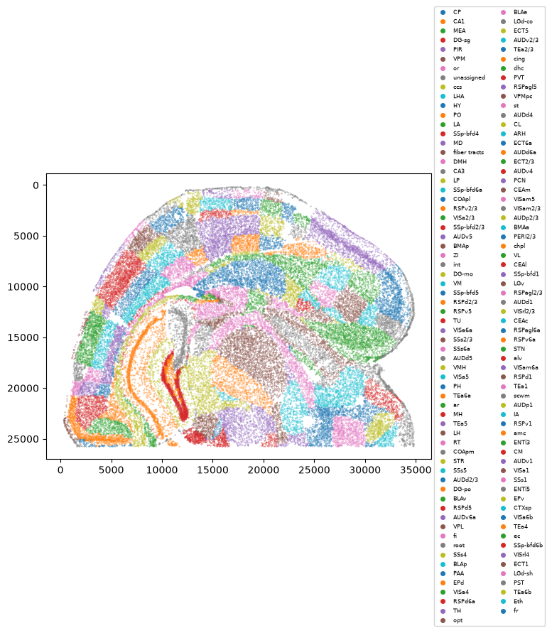
Cells coloured by structure#
keep = acronym.value_counts()
keep = keep[keep >= 50].index                       # a legend of singletons reads as noise
fig, ax = plt.subplots(figsize=(7, 6))
for region in keep:
    m = (acronym == region).to_numpy()
    ax.scatter(xy[m, 0], xy[m, 1], s=0.08, label=region)
ax.invert_yaxis(); ax.set_aspect('equal')
ax.legend(handles=[Line2D([], [], marker='o', ls='', ms=4, color=h.get_facecolor()[0], label=r)
                   for r, h in zip(keep, ax.collections, strict=True)],
          fontsize=6, ncol=2, loc='center left', bbox_to_anchor=(1, 0.5))
<matplotlib.legend.Legend at 0x7f1ad4147230>