Placing a MERFISH section in the Allen CCF#
The same volume-to-section fit as the STARmap notebook, on a
denser section and a finer raster. It is the simpler of the two to write: this section needs
no anisotropic initialisation, so initial_slice, initial_rotation and initial_scale say
the whole starting guess and initial_affine never appears.
STalign’s own version of this analysis: merfish-allen3Datlas-alignment.
Inputs#
Cells as a points element, the atlas and its annotation volume as 3D images. The physical placement lives on the elements, so nothing downstream builds coordinate axes by hand.
import nrrd, numpy as np, pandas as pd, spatialdata as sd
from spatialdata.models import Image3DModel, PointsModel
from spatialdata.transformations import Scale, Sequence, Translation

cells = pd.read_csv('merfish_data/datasets_mouse_brain_map_BrainReceptorShowcase'
                    '_Slice1_Replicate1_cell_metadata_S1R1.csv.gz')
xy = np.c_[cells['center_x'], cells['center_y']].astype(float)

atlas, hdr = nrrd.read('ara_nissl_50.nrrd')       # (z, y, x)
labels, _ = nrrd.read('annotation_50.nrrd')       # same frame, integer structure ids
voxel = tuple(np.diag(hdr['space directions']))

# The second channel is not decoration: the solver regresses the deformed reference onto the
# section before measuring the match, so one channel fits `a + b*I` and two fit
# `a + b*I + c*(I - mean I)**2`. A regression absorbs a rescaling of its input; it cannot
# invent a channel it was never handed.
def reference_channels(volume):
    v = volume[None] / np.mean(np.abs(volume))
    return np.concatenate([v, (v - v.mean()) ** 2])

sdata = sd.SpatialData(
    points={'cells': PointsModel.parse(xy)},
    images={'atlas': Image3DModel.parse(
        reference_channels(atlas.astype(float)), dims=('c', 'z', 'y', 'x'),
        transformations={'global': Sequence([
            Scale(list(voxel), axes=('z', 'y', 'x')),
            Translation(-(np.asarray(atlas.shape) - 1) * np.asarray(voxel) / 2,
                        axes=('z', 'y', 'x')),
        ])},
    )},
)
sdata
SpatialData object
├── Images
│     └── 'atlas': DataArray[czyx] (2, 264, 160, 228)
└── Points
      └── 'cells': DataFrame with shape: (<Delayed>, 2) (2D points)
with coordinate systems:
    ▸ 'global', with elements:
        atlas (Images), cells (Points)
The section#
rasterize_points turns the centroids into a density image: each cell deposits unit mass
bilinearly, blurred once per scale, so total intensity is exactly the cell count.
from squidpy.experimental.im import rasterize_points, sample_volume

rasterize_points(sdata, points_key='cells', dx=10.0, blur=1.0, key_added='section')
sdata['section']
<xarray.DataArray 'image' (c: 1, y: 696, x: 995)> Size: 6MB
dask.array<array, shape=(1, 696, 995), dtype=float64, chunksize=(1, 696, 995), chunktype=numpy.ndarray>
Coordinates:
  * c        (c) int64 8B 0
  * y        (y) float64 6kB 0.5 1.5 2.5 3.5 4.5 ... 692.5 693.5 694.5 695.5
  * x        (x) float64 8kB 0.5 1.5 2.5 3.5 4.5 ... 991.5 992.5 993.5 994.5
Attributes:
transform: {'global': Sequence \n Scale (y, x)\n [10. 10.]\n ...Putting the section on the scale the solver’s parameters assume#
sigmaM, sigmaA, sigmaB, muA and muB are all in the target’s intensity units, and
upstream states its values against a mean-normalised section. Handing over the raw raster
instead leaves every one of those widths wrong by the raster’s own mean – which for a dx=10
raster is a factor of nine, enough to flatten the artifact/background/matching split into
near-constants and leave the fit with almost no gradient to descend.
from spatialdata.models import Image2DModel
from spatialdata.transformations import get_transformation

def mean_normalised(sdata, key):
    element = sdata.images[key]
    values = np.asarray(element)
    sdata.images[key] = Image2DModel.parse(
        values / np.abs(values).mean(), dims=('c', 'y', 'x'),
        transformations={'global': get_transformation(element, 'global')},
    )

mean_normalised(sdata, 'section')
section = np.asarray(sdata['section']).squeeze()
print(f'section now spans {section.min():.2f} to {section.max():.2f}, mean {section.mean():.2f}')
section now spans 0.00 to 7.35, mean 1.00
The fit#
The section is close to coronal and close to atlas scale, so the initialisation is three numbers: which slice to centre on, how far to rotate in plane, and one uniform scale.
Upstream also nudges the starting translation by a single landmark pair, worth about 42 um in
x and 7 um in y – four pixels and under one. That is an initialisation, not an answer, and
the next cell checks the initialisation directly, so it is left out here rather than
reintroducing a hand-built affine to carry it.
from squidpy.experimental.tl import stalign_align_volume

slice_index, rotation, scale = 177, 0.0, 0.9

# Upstream's own values, now that the section is on the scale they were written for. One
# channel, not three: upstream passes `muA=[3, 3, 3]` against a single-channel target and sums
# over the broadcast axis, making its effective widths sigma/sqrt(3) -- divergence D13.
#
# `a` and `sigmaR` are set rather than left to the defaults, from a 3x3 sweep over
# a in {250, 500, 1000} and sigmaR in {1e5, 1e6, 1e7}. A 250 um kernel resolves the
# hippocampal arcs and cortical laminae visibly better than the 500 um default, and at
# sigmaR 1e5 it is the only sweep point that keeps every region the default assigns --
# 163 against 161, none lost -- while agreeing with it on 86% of the 78329 cells. The
# looser sigmaR 1e7 looked sharper still but dropped all of lateral auditory cortex
# (AUDv5, AUDpo5, AUDp1 and six more) to zero cells, which reads as the section's edge
# leaving the annotated volume rather than a real difference in detail.
#
# Upstream's `LDDMM_3D_to_slice` declares sigmaR 1e8, which weights the regulariser so
# weakly against squidpy's corrected rank-3 energy that the velocity field grows
# unchecked; 1e5 here is two orders below squidpy's own 1e6 default, not near upstream's.
SOLVER = dict(a=250.0, sigmaR=1e5, nt=4, sigmaM=2.0, sigmaA=2.0, sigmaB=2.0, muA=[3.0], muB=[0.0])
fit = stalign_align_volume(
    sdata, image_key=('atlas', 'section'), niter=2000,
    initial_slice=slice_index, initial_rotation=rotation, initial_scale=scale, **SOLVER,
)
print(f'{fit.n_iter} iterations, objective '
      f'{float(fit.energies[0]):.0f} -> {float(fit.energies[-1]):.0f}')
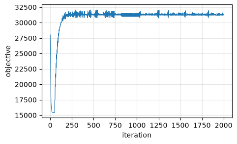
2000 iterations, objective 28029 -> 31302
Convergence#
import matplotlib.pyplot as plt

energies = np.asarray(fit.energies)[: fit.n_iter]
plt.figure(figsize=(5, 3))
plt.plot(energies, lw=0.8)
plt.xlabel('iteration'); plt.ylabel('objective'); plt.grid(alpha=0.3)
Where each cell lands#
StalignFit.transform_points maps (x, y) section coordinates to (x, y, z) reference coordinates, evaluated at
each point rather than at the nearest raster cell. sample_volume then reads the annotation
volume there – order=0 because structure ids must not be interpolated.
coords = np.asarray(fit.transform_points(xy))  # (N, 3), (x, y, z) in microns
structure_id = sample_volume(labels, coords, axes=fit.ref_axes, order=0).astype(int)

print(f'{len(coords)} cells placed, {np.unique(structure_id).size} distinct structures, '
      f'{100 * (structure_id == 0).mean():.1f}% outside any annotated structure')
print(f'depth (z) spans {coords[:, 2].min():.0f} to {coords[:, 2].max():.0f} um')
78329 cells placed, 162 distinct structures, 3.5% outside any annotated structure
depth (z) spans 2066 to 2505 um
Structure ids become acronyms through the Allen ontology.
ontology = pd.read_csv('allen_ontology.csv').set_index('id')['acronym']
acronym = pd.Series(structure_id).map(ontology).fillna('unassigned')
acronym.value_counts().head(12)
CA1           4559
MRN           4072
MB            2870
unassigned    2734
PG            2724
SCig          2675
SCiw          2409
DG-mo         2276
PAG           2253
ProS          2222
VISp2/3       1808
POST          1634
Name: count, dtype: int64
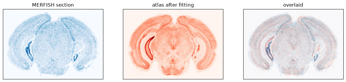
The aligned atlas over the section#
import matplotlib as mpl
from matplotlib.lines import Line2D

def atlas_at(result):
    plane = np.moveaxis(np.asarray(result.deformation_grid()), 0, -1)[0]
    sampled = sample_volume(atlas, plane.reshape(-1, 3)[:, ::-1], axes=result.ref_axes)
    return sampled.reshape(plane.shape[:2])

section = np.asarray(sdata['section']).squeeze()
fig, ax = plt.subplots(1, 3, figsize=(15, 5))
ax[0].imshow(section, cmap=mpl.cm.Blues)
ax[1].imshow(atlas_at(fit), cmap=mpl.cm.Reds)
ax[2].imshow(section, cmap=mpl.cm.Blues, alpha=0.9)
ax[2].imshow(atlas_at(fit), cmap=mpl.cm.Reds, alpha=0.3)
for a, t in zip(ax, ('MERFISH section', 'atlas after fitting', 'overlaid'), strict=True):
    a.set_title(t); a.set_xticks([]); a.set_yticks([])
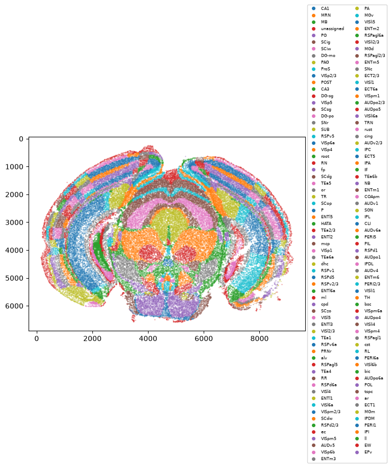
Cells coloured by structure#
keep = acronym.value_counts()
keep = keep[keep >= 50].index                       # a legend of singletons reads as noise
fig, ax = plt.subplots(figsize=(7, 6))
for region in keep:
    m = (acronym == region).to_numpy()
    ax.scatter(xy[m, 0], xy[m, 1], s=0.08, label=region)
ax.invert_yaxis(); ax.set_aspect('equal')
ax.legend(handles=[Line2D([], [], marker='o', ls='', ms=4, color=h.get_facecolor()[0], label=r)
                   for r, h in zip(keep, ax.collections, strict=True)],
          fontsize=6, ncol=2, loc='center left', bbox_to_anchor=(1, 0.5))
<matplotlib.legend.Legend at 0x7fb084905fd0>