Performance comparison of inference on cell cycle

Notebook compares metrics for velocity, latent time and GRN inference across different methods applied to cell cycle data.

Library imports

import numpy as np
import pandas as pd

import matplotlib.pyplot as plt
import mplscience
import seaborn as sns

from rgv_tools import DATA_DIR, FIG_DIR

General settings

DATASET = "cell_cycle"

SAVE_FIGURES = True
if SAVE_FIGURES:
    (FIG_DIR / DATASET).mkdir(parents=True, exist_ok=True)

FIGURE_FORMATE = "svg"

Constants

NN_SCALE = [10, 30, 50, 70, 90, 100]
VELO_METHODS = ["regvelo", "velovi"]

VELO_METHOD_PALETTE = {
    "regvelo": "#0173b2",
    "velovi": "#de8f05",
}

Velocity loading

## Velocity
confi_df = []

for scale in NN_SCALE:
    df = pd.read_parquet(DATA_DIR / "results" / f"regvelo_confidence_velocity_{scale}.parquet")
    df["scale"] = scale
    confi_df.append(df)

confi_df = pd.concat(confi_df, axis=0)

Confidence

confi_df

	velocity_consistency	Dataset	Method	scale
0	0.941898	Cell cycle	regvelo	10
1	0.951289	Cell cycle	regvelo	10
2	0.904966	Cell cycle	regvelo	10
3	0.541206	Cell cycle	regvelo	10
4	0.886754	Cell cycle	regvelo	10
...	...	...	...	...
1141	0.981466	Cell cycle	regvelo	100
1142	0.918879	Cell cycle	regvelo	100
1143	0.921603	Cell cycle	regvelo	100
1144	0.963663	Cell cycle	regvelo	100
1145	0.952200	Cell cycle	regvelo	100

6876 rows × 4 columns

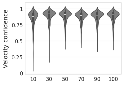
with mplscience.style_context():
    sns.set_style(style="whitegrid")
    fig, ax = plt.subplots(figsize=(4, 3), sharey=True)
    sns.violinplot(
        data=confi_df,
        ax=ax,
        # orient="h",
        x="scale",
        y="velocity_consistency",
        color="grey",
        order=NN_SCALE,
    )
    # plt.legend(title='', loc='lower center', bbox_to_anchor=(0.5, -0.6), ncol=3)
    ax.set_yticks([0, 0.25, 0.5, 0.75, 1])
    ax.set_yticklabels([0, 0.25, 0.5, 0.75, 1])
    ax.set_ylabel("Velocity confidence", fontsize=14)
    ax.set_xlabel("")
    plt.show()

    if SAVE_FIGURES:
        fig.savefig(FIG_DIR / "velocity_confidence_compare.svg", format="svg", transparent=True, bbox_inches="tight")
    plt.show()

Compare on each level

confi_dfs = []
for scale in NN_SCALE:
    confi_df = []
    for method in VELO_METHODS:
        df = pd.read_parquet(DATA_DIR / "results" / f"{method}_confidence_velocity_{scale}_nn30.parquet")
        confi_df.append(df)

    confi_df = pd.concat(confi_df, axis=0)
    confi_df["Scale"] = scale
    confi_dfs.append(confi_df)

confi_dfs = pd.concat(confi_dfs)

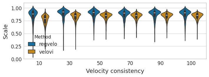
with mplscience.style_context():
    sns.set_style(style="whitegrid")
    fig, ax = plt.subplots(figsize=(8, 2.5))
    sns.violinplot(
        data=confi_dfs,
        y="velocity_consistency",
        x="Scale",
        hue="Method",
        hue_order=["regvelo", "velovi"],
        palette=VELO_METHOD_PALETTE,
        ax=ax,
    )

    ax.set(
        xlabel="Velocity consistency",
        ylabel="Scale",
        yticks=ax.get_yticks(),
    )
    ax.set_ylim(0, 1.1)

    fig.savefig(
        FIG_DIR / "velocity_confidence.svg",
        format="svg",
        transparent=True,
        bbox_inches="tight",
    )

    plt.show()

confi_dfs_velo = confi_dfs.copy()

confi_dfs = []
for scale in NN_SCALE:
    confi_df = []
    for method in VELO_METHODS:
        df = pd.read_parquet(DATA_DIR / "results" / f"{method}_confidence_time_{scale}_nn30.parquet")
        confi_df.append(df)

    confi_df = pd.concat(confi_df, axis=0)
    confi_df["Scale"] = scale
    confi_dfs.append(confi_df)

confi_dfs = pd.concat(confi_dfs)

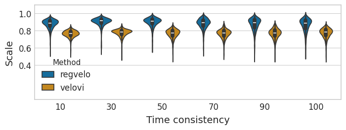
with mplscience.style_context():
    sns.set_style(style="whitegrid")
    fig, ax = plt.subplots(figsize=(8, 2.5))
    sns.violinplot(
        data=confi_dfs,
        y="fit_t_consistency",
        x="Scale",
        hue="Method",
        hue_order=["regvelo", "velovi"],
        palette=VELO_METHOD_PALETTE,
        ax=ax,
    )

    ax.set(
        xlabel="Time consistency",
        ylabel="Scale",
        yticks=ax.get_yticks(),
    )
    ax.set_ylim(0, 1.1)

    fig.savefig(
        FIG_DIR / "time_confidence.svg",
        format="svg",
        transparent=True,
        bbox_inches="tight",
    )

    plt.show()

confi_dfs_time = confi_dfs.copy()

confi_dfs_velo_ratio = []
for scale in np.unique(confi_dfs_velo["Scale"]):
    dat = pd.DataFrame()
    repeat = int(int(np.sum(confi_dfs_velo["Scale"] == scale)) / 2)
    dat["Scale"] = [scale] * repeat
    velo_reg = confi_dfs_velo.loc[
        (confi_dfs_velo["Scale"] == scale) * (confi_dfs_velo["Method"] == "regvelo"), "velocity_consistency"
    ]
    velo_vi = confi_dfs_velo.loc[
        (confi_dfs_velo["Scale"] == scale) * (confi_dfs_velo["Method"] == "velovi"), "velocity_consistency"
    ]
    dat["Ratio"] = velo_reg / velo_vi
    dat["Class"] = ["velocity"] * repeat
    confi_dfs_velo_ratio.append(dat)

confi_dfs_time_ratio = []
for scale in np.unique(confi_dfs_time["Scale"]):
    dat = pd.DataFrame()
    repeat = int(int(np.sum(confi_dfs_time["Scale"] == scale)) / 2)
    dat["Scale"] = [scale] * repeat
    time_reg = confi_dfs_time.loc[
        (confi_dfs_time["Scale"] == scale) * (confi_dfs_time["Method"] == "regvelo"), "fit_t_consistency"
    ]
    time_vi = confi_dfs_time.loc[
        (confi_dfs_time["Scale"] == scale) * (confi_dfs_time["Method"] == "velovi"), "fit_t_consistency"
    ]
    dat["Ratio"] = time_reg / time_vi
    dat["Class"] = ["time"] * repeat
    confi_dfs_time_ratio.append(dat)

confi_dfs_velo_ratio = pd.concat(confi_dfs_velo_ratio)
confi_dfs_time_ratio = pd.concat(confi_dfs_time_ratio)
confi_df_all = pd.concat([confi_dfs_velo_ratio, confi_dfs_time_ratio])

confi_df_all

	Scale	Ratio	Class
0	10	1.111715	velocity
1	10	1.087845	velocity
2	10	1.113454	velocity
3	10	0.976719	velocity
4	10	1.001859	velocity
...	...	...	...
1141	100	1.124350	time
1142	100	1.139394	time
1143	100	1.109670	time
1144	100	1.142055	time
1145	100	1.176460	time

13752 rows × 3 columns

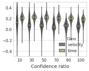
confi_df_all["Scale"] = confi_df_all["Scale"].astype(str)

confi_df_all["Ratio"] = confi_df_all["Ratio"].astype(np.float32)

confi_df_all["Ratio"] = np.log2(confi_df_all["Ratio"])

custom_palette = {
    "velocity": "#7D7C78",  # Elegant blue (colorblind-friendly)
    "time": "#BCAE6C",  # Gold-orange (also friendly and high contrast)
}

with mplscience.style_context():
    sns.set_style(style="whitegrid")
    fig, ax = plt.subplots(figsize=(4, 3), sharey=True)
    sns.violinplot(
        data=confi_df_all,
        ax=ax,
        y="Ratio",
        x="Scale",
        hue="Class",
        palette=custom_palette,
    )
    # plt.legend(title='', loc='lower center', bbox_to_anchor=(0.5, -0.6), ncol=3)
    ax.set_ylim(-0.5, 0.5)
    # ax.set_yticklabels([0,0.25, 0.5, 0.75,1]);
    ax.set_xlabel("Confidence ratio", fontsize=14)
    ax.set_ylabel("")
    plt.show()

    if SAVE_FIGURES:
        fig.savefig(FIG_DIR / "confi_all_kinetics.svg", format="svg", transparent=True, bbox_inches="tight")
    plt.show()