Benchmark transcription rate prediction#
Notebooks for benchmarking transcription rate prediction on metabolic labelled cell cycle datasets
Library imports#
import numpy as np
import pandas as pd
import scipy
import torch
from scipy.stats import ttest_ind

import matplotlib.pyplot as plt
import mplscience
import seaborn as sns

import scanpy as sc
from regvelo import REGVELOVI

from rgv_tools import DATA_DIR, FIG_DIR
from rgv_tools.plotting._significance import add_significance, get_significance
Constants#
DATASET = "cell_cycle_rpe1"
SAVE_DATA = True
SAVE_FIGURES = True
if SAVE_DATA:
    (DATA_DIR / DATASET / "processed").mkdir(parents=True, exist_ok=True)
    (FIG_DIR / DATASET).mkdir(parents=True, exist_ok=True)
Data loading#
adata = sc.read_h5ad(DATA_DIR / DATASET / "processed" / "adata_processed.h5ad")
alpha = pd.read_csv(
    DATA_DIR / DATASET / "raw" / "aax3072_table-s1.csv", index_col=2, header=1
)  # downloaded from the supplementary of https://www.science.org/doi/10.1126/science.aax3072
alpha = alpha.filter(regex="^norm_kappa_")
alpha
| norm_kappa_000 | norm_kappa_001 | norm_kappa_002 | norm_kappa_003 | norm_kappa_004 | norm_kappa_005 | norm_kappa_006 | norm_kappa_007 | norm_kappa_008 | norm_kappa_009 | ... | norm_kappa_291 | norm_kappa_292 | norm_kappa_293 | norm_kappa_294 | norm_kappa_295 | norm_kappa_296 | norm_kappa_297 | norm_kappa_298 | norm_kappa_299 | norm_kappa_300 | |
|---|---|---|---|---|---|---|---|---|---|---|---|---|---|---|---|---|---|---|---|---|---|
| gene_symbol | |||||||||||||||||||||
| UBALD2 | 1.179867 | 1.179867 | 1.179867 | 1.179867 | 1.179867 | 1.179867 | 1.165868 | 1.165868 | 1.124469 | 1.124469 | ... | 1.393822 | 1.389139 | 1.387780 | 1.387780 | 1.387780 | 1.387780 | 1.387780 | 1.387780 | 1.387780 | 1.387780 |
| LMNB2 | 0.118109 | 0.118109 | 0.118109 | 0.091849 | 0.091849 | 0.091849 | 0.091849 | 0.091849 | 0.091849 | 0.016334 | ... | 0.328110 | 0.328110 | 0.328110 | 0.328110 | 0.328110 | 0.320427 | 0.320427 | 0.320427 | 0.304818 | 0.304818 |
| SOGA1 | 0.088258 | 0.088258 | 0.020962 | 0.020962 | 0.020962 | 0.020962 | 0.012680 | 0.012680 | 0.012680 | 0.012680 | ... | 0.518963 | 0.470260 | 0.432552 | 0.432552 | 0.397859 | 0.397859 | 0.381700 | 0.381700 | 0.381700 | 0.381700 |
| PPIP5K2 | 0.108402 | 0.071083 | 0.071083 | 0.071083 | 0.071083 | 0.071083 | 0.071083 | 0.071083 | 0.071083 | 0.043664 | ... | 0.593905 | 0.593905 | 0.457897 | 0.457897 | 0.457897 | 0.457897 | 0.457897 | 0.447648 | 0.447648 | 0.447648 |
| PTPRJ | 1.002031 | 1.002031 | 1.002031 | 1.002031 | 1.002031 | 1.002031 | 1.002031 | 1.002031 | 0.888077 | 0.861586 | ... | 1.276865 | 1.270956 | 1.266449 | 1.266449 | 1.266449 | 1.251248 | 1.251248 | 1.251248 | 1.251248 | 1.251248 |
| ... | ... | ... | ... | ... | ... | ... | ... | ... | ... | ... | ... | ... | ... | ... | ... | ... | ... | ... | ... | ... | ... |
| SGMS2 | -1.192674 | -1.192674 | -1.192674 | -1.192674 | -1.208510 | -1.224163 | -1.208510 | -1.208510 | -1.208510 | -1.208510 | ... | -0.453817 | -0.479000 | -0.479000 | -0.479000 | -0.479000 | -0.504759 | -0.504759 | -0.542460 | -0.542460 | -0.549843 |
| PMAIP1 | -0.183754 | -0.183754 | -0.183754 | -0.183754 | -0.183754 | -0.183754 | -0.183754 | -0.183754 | -0.184812 | -0.223222 | ... | -0.042112 | -0.044428 | -0.044428 | -0.060940 | -0.060940 | -0.060940 | -0.080172 | -0.080172 | -0.080172 | -0.080172 |
| DHCR24 | -0.450735 | -0.450735 | -0.450735 | -0.450735 | -0.450735 | -0.450735 | -0.450735 | -0.450735 | -0.484615 | -0.493553 | ... | -0.320440 | -0.329280 | -0.329280 | -0.329280 | -0.329280 | -0.329280 | -0.330464 | -0.330464 | -0.376690 | -0.384143 |
| POLE | -0.529833 | -0.529833 | -0.529833 | -0.575677 | -0.575677 | -0.575677 | -0.575677 | -0.575677 | -0.603306 | -0.603306 | ... | -0.412773 | -0.420573 | -0.420573 | -0.420573 | -0.488070 | -0.506770 | -0.506770 | -0.506770 | -0.506770 | -0.506770 |
| ANKRD36C | -0.432021 | -0.432021 | -0.432021 | -0.432021 | -0.432021 | -0.432021 | -0.447457 | -0.447457 | -0.467636 | -0.498658 | ... | -0.221038 | -0.256899 | -0.256899 | -0.274694 | -0.274694 | -0.274694 | -0.274694 | -0.274694 | -0.274694 | -0.274694 |
528 rows × 301 columns
alpha.columns = np.array([i.replace("norm_kappa_", "") for i in alpha.columns], dtype=np.float32)
pos = adata.obs["cell_cycle_position"].unique()
GEX = []

for i in pos:
    gex = adata[adata.obs["cell_cycle_position"] == i].X.A.mean(axis=0)
    GEX.append(gex)
GEX = np.array(GEX).T
GEX = pd.DataFrame(GEX, index=adata.var_names.tolist())
GEX
| 0 | 1 | 2 | 3 | 4 | 5 | 6 | 7 | 8 | 9 | ... | 280 | 281 | 282 | 283 | 284 | 285 | 286 | 287 | 288 | 289 | |
|---|---|---|---|---|---|---|---|---|---|---|---|---|---|---|---|---|---|---|---|---|---|
| DEPDC1 | 0.161310 | 0.328377 | 0.126236 | 0.000000 | 0.445840 | 0.742209 | 0.684013 | 0.317394 | 0.509439 | 0.180416 | ... | 0.337324 | 0.523796 | 1.649758 | 0.000000 | 0.357087 | 1.076477 | 0.000000 | 0.000000 | 0.000000 | 0.000000 |
| TRIO | 1.981804 | 1.515634 | 1.730185 | 2.096108 | 1.660738 | 1.462572 | 1.611647 | 2.059388 | 2.121015 | 1.883820 | ... | 1.791328 | 2.165788 | 0.876263 | 2.176786 | 0.636869 | 2.048151 | 2.324368 | 2.076471 | 2.328215 | 1.574311 |
| ADAMTS6 | 1.273340 | 1.115689 | 0.793328 | 0.815586 | 0.724796 | 0.495016 | 0.865061 | 1.060191 | 1.100434 | 0.940455 | ... | 1.411591 | 1.539369 | 0.876263 | 1.219352 | 0.525509 | 1.306756 | 1.440009 | 1.383749 | 0.000000 | 0.000000 |
| POLQ | 0.220024 | 0.093262 | 0.655998 | 0.120990 | 0.369249 | 0.329390 | 0.096619 | 0.529976 | 0.502093 | 0.098990 | ... | 0.309368 | 0.322715 | 1.888225 | 0.260449 | 0.000000 | 0.230847 | 0.470612 | 0.000000 | 0.320231 | 1.574311 |
| SYNE2 | 0.456051 | 0.121919 | 0.452270 | 0.317492 | 0.821573 | 0.516719 | 0.412208 | 0.884521 | 0.536059 | 0.589152 | ... | 0.966696 | 0.376468 | 1.336004 | 1.522307 | 0.000000 | 0.851015 | 0.000000 | 0.691451 | 0.320231 | 1.069426 |
| ... | ... | ... | ... | ... | ... | ... | ... | ... | ... | ... | ... | ... | ... | ... | ... | ... | ... | ... | ... | ... | ... |
| MANCR | 1.107140 | 0.836700 | 0.756655 | 0.554660 | 0.632607 | 1.029576 | 0.840048 | 1.151329 | 1.099359 | 0.443124 | ... | 0.780349 | 1.278557 | 0.000000 | 1.791222 | 0.335229 | 0.574196 | 1.046393 | 1.096350 | 0.320231 | 0.000000 |
| MTATP6P1 | 2.288898 | 2.405079 | 2.159031 | 2.227160 | 2.321663 | 2.195483 | 2.659615 | 2.515312 | 2.502668 | 2.483743 | ... | 2.828326 | 2.249292 | 2.709321 | 2.271032 | 2.617242 | 2.023398 | 1.604221 | 2.830018 | 2.296170 | 2.158117 |
| MIR100HG | 1.508564 | 1.982803 | 1.997843 | 2.543906 | 2.180073 | 2.280532 | 2.287652 | 1.908947 | 1.789601 | 2.454187 | ... | 1.833768 | 2.028000 | 0.876263 | 1.520726 | 2.845396 | 2.284718 | 1.737294 | 1.943000 | 2.607786 | 1.908226 |
| SNHG1 | 1.340924 | 0.865615 | 0.407378 | 0.911950 | 1.100356 | 0.833532 | 1.037473 | 0.792740 | 1.336403 | 0.926061 | ... | 0.710278 | 0.952297 | 1.336004 | 0.341737 | 0.692316 | 0.947387 | 1.179466 | 1.096350 | 0.653094 | 1.908226 |
| SNHG19 | 0.349352 | 0.636762 | 0.260200 | 0.517246 | 0.360954 | 0.710418 | 0.619507 | 0.398636 | 0.000000 | 0.374218 | ... | 0.149108 | 0.376468 | 0.000000 | 0.685875 | 0.357087 | 0.919150 | 0.575781 | 0.000000 | 0.792144 | 0.000000 |
141 rows × 290 columns
gs = list(set(alpha.index.tolist()).intersection(adata.var_names.tolist()))
GEX.loc[gs, :]
| 0 | 1 | 2 | 3 | 4 | 5 | 6 | 7 | 8 | 9 | ... | 280 | 281 | 282 | 283 | 284 | 285 | 286 | 287 | 288 | 289 | |
|---|---|---|---|---|---|---|---|---|---|---|---|---|---|---|---|---|---|---|---|---|---|
| PAPPA | 0.236026 | 0.595305 | 0.754837 | 0.815792 | 0.590248 | 0.554654 | 0.354364 | 0.417110 | 0.374995 | 0.716544 | ... | 0.861246 | 0.409270 | 0.876263 | 0.000000 | 0.370403 | 0.388174 | 0.000000 | 0.000000 | 0.792144 | 0.000000 |
| RIMS2 | 0.000000 | 0.330232 | 0.247463 | 0.379518 | 0.510151 | 0.191398 | 0.000000 | 0.603839 | 0.530653 | 0.054663 | ... | 0.559815 | 0.573492 | 0.000000 | 0.430828 | 0.370403 | 0.388174 | 0.000000 | 0.691451 | 0.513865 | 0.000000 |
| MIR100HG | 1.508564 | 1.982803 | 1.997843 | 2.543906 | 2.180073 | 2.280532 | 2.287652 | 1.908947 | 1.789601 | 2.454187 | ... | 1.833768 | 2.028000 | 0.876263 | 1.520726 | 2.845396 | 2.284718 | 1.737294 | 1.943000 | 2.607786 | 1.908226 |
| G2E3 | 0.236026 | 0.113038 | 0.136443 | 0.140211 | 0.337680 | 0.120133 | 0.133690 | 0.392664 | 0.870752 | 0.156803 | ... | 0.428223 | 0.381109 | 2.080633 | 0.742809 | 0.357087 | 0.000000 | 0.470612 | 0.000000 | 0.513865 | 1.574311 |
| AURKA | 0.851758 | 0.219980 | 0.172232 | 0.104639 | 0.240032 | 0.335769 | 0.474674 | 0.418812 | 0.273523 | 0.318951 | ... | 0.646679 | 0.824949 | 0.876263 | 0.000000 | 0.895912 | 1.030397 | 0.864525 | 0.000000 | 0.000000 | 1.069426 |
| ... | ... | ... | ... | ... | ... | ... | ... | ... | ... | ... | ... | ... | ... | ... | ... | ... | ... | ... | ... | ... | ... |
| CENPF | 1.120599 | 0.872054 | 0.628304 | 0.371293 | 0.910407 | 1.810582 | 1.590818 | 1.217998 | 1.629507 | 1.057226 | ... | 0.805158 | 1.354087 | 1.649758 | 1.357588 | 1.873811 | 1.849402 | 1.826995 | 1.788931 | 0.471913 | 2.524307 |
| MCM10 | 0.129327 | 0.107488 | 0.685333 | 0.266811 | 0.399895 | 0.390223 | 0.047354 | 0.330642 | 0.387730 | 0.176696 | ... | 0.342713 | 0.135464 | 0.000000 | 0.000000 | 0.000000 | 0.230847 | 0.000000 | 0.000000 | 1.524149 | 0.000000 |
| KPNA2 | 0.710659 | 0.691963 | 0.619302 | 0.493050 | 0.431500 | 0.712793 | 0.647899 | 0.648701 | 0.669845 | 0.639119 | ... | 0.473450 | 0.930215 | 2.080633 | 0.803296 | 0.370403 | 1.600532 | 1.545007 | 0.691451 | 0.000000 | 1.069426 |
| PTTG1 | 1.176973 | 1.258670 | 1.011124 | 0.911626 | 0.870235 | 1.471961 | 1.531632 | 0.854305 | 1.377528 | 1.618404 | ... | 0.479520 | 1.270856 | 2.241926 | 1.539767 | 0.860738 | 1.503640 | 1.046393 | 1.383749 | 0.513865 | 1.069426 |
| PKMYT1 | 0.940430 | 0.351545 | 0.664576 | 0.297624 | 0.800065 | 0.745133 | 0.171471 | 0.848509 | 0.276872 | 0.296031 | ... | 1.045587 | 0.669761 | 0.000000 | 0.430828 | 0.000000 | 0.851015 | 0.288744 | 0.691451 | 0.000000 | 1.069426 |
75 rows × 290 columns
GEX.columns = pos
GEX
| 230.0 | 66.0 | 109.0 | 85.0 | 177.0 | 49.0 | 55.0 | 196.0 | 254.0 | 60.0 | ... | 242.0 | 259.0 | 21.0 | 247.0 | 42.0 | 287.0 | 296.0 | 232.0 | 106.0 | 4.0 | |
|---|---|---|---|---|---|---|---|---|---|---|---|---|---|---|---|---|---|---|---|---|---|
| DEPDC1 | 0.161310 | 0.328377 | 0.126236 | 0.000000 | 0.445840 | 0.742209 | 0.684013 | 0.317394 | 0.509439 | 0.180416 | ... | 0.337324 | 0.523796 | 1.649758 | 0.000000 | 0.357087 | 1.076477 | 0.000000 | 0.000000 | 0.000000 | 0.000000 |
| TRIO | 1.981804 | 1.515634 | 1.730185 | 2.096108 | 1.660738 | 1.462572 | 1.611647 | 2.059388 | 2.121015 | 1.883820 | ... | 1.791328 | 2.165788 | 0.876263 | 2.176786 | 0.636869 | 2.048151 | 2.324368 | 2.076471 | 2.328215 | 1.574311 |
| ADAMTS6 | 1.273340 | 1.115689 | 0.793328 | 0.815586 | 0.724796 | 0.495016 | 0.865061 | 1.060191 | 1.100434 | 0.940455 | ... | 1.411591 | 1.539369 | 0.876263 | 1.219352 | 0.525509 | 1.306756 | 1.440009 | 1.383749 | 0.000000 | 0.000000 |
| POLQ | 0.220024 | 0.093262 | 0.655998 | 0.120990 | 0.369249 | 0.329390 | 0.096619 | 0.529976 | 0.502093 | 0.098990 | ... | 0.309368 | 0.322715 | 1.888225 | 0.260449 | 0.000000 | 0.230847 | 0.470612 | 0.000000 | 0.320231 | 1.574311 |
| SYNE2 | 0.456051 | 0.121919 | 0.452270 | 0.317492 | 0.821573 | 0.516719 | 0.412208 | 0.884521 | 0.536059 | 0.589152 | ... | 0.966696 | 0.376468 | 1.336004 | 1.522307 | 0.000000 | 0.851015 | 0.000000 | 0.691451 | 0.320231 | 1.069426 |
| ... | ... | ... | ... | ... | ... | ... | ... | ... | ... | ... | ... | ... | ... | ... | ... | ... | ... | ... | ... | ... | ... |
| MANCR | 1.107140 | 0.836700 | 0.756655 | 0.554660 | 0.632607 | 1.029576 | 0.840048 | 1.151329 | 1.099359 | 0.443124 | ... | 0.780349 | 1.278557 | 0.000000 | 1.791222 | 0.335229 | 0.574196 | 1.046393 | 1.096350 | 0.320231 | 0.000000 |
| MTATP6P1 | 2.288898 | 2.405079 | 2.159031 | 2.227160 | 2.321663 | 2.195483 | 2.659615 | 2.515312 | 2.502668 | 2.483743 | ... | 2.828326 | 2.249292 | 2.709321 | 2.271032 | 2.617242 | 2.023398 | 1.604221 | 2.830018 | 2.296170 | 2.158117 |
| MIR100HG | 1.508564 | 1.982803 | 1.997843 | 2.543906 | 2.180073 | 2.280532 | 2.287652 | 1.908947 | 1.789601 | 2.454187 | ... | 1.833768 | 2.028000 | 0.876263 | 1.520726 | 2.845396 | 2.284718 | 1.737294 | 1.943000 | 2.607786 | 1.908226 |
| SNHG1 | 1.340924 | 0.865615 | 0.407378 | 0.911950 | 1.100356 | 0.833532 | 1.037473 | 0.792740 | 1.336403 | 0.926061 | ... | 0.710278 | 0.952297 | 1.336004 | 0.341737 | 0.692316 | 0.947387 | 1.179466 | 1.096350 | 0.653094 | 1.908226 |
| SNHG19 | 0.349352 | 0.636762 | 0.260200 | 0.517246 | 0.360954 | 0.710418 | 0.619507 | 0.398636 | 0.000000 | 0.374218 | ... | 0.149108 | 0.376468 | 0.000000 | 0.685875 | 0.357087 | 0.919150 | 0.575781 | 0.000000 | 0.792144 | 0.000000 |
141 rows × 290 columns
alpha = alpha.loc[:, pos]
alpha
| 230.0 | 66.0 | 109.0 | 85.0 | 177.0 | 49.0 | 55.0 | 196.0 | 254.0 | 60.0 | ... | 242.0 | 259.0 | 21.0 | 247.0 | 42.0 | 287.0 | 296.0 | 232.0 | 106.0 | 4.0 | |
|---|---|---|---|---|---|---|---|---|---|---|---|---|---|---|---|---|---|---|---|---|---|
| gene_symbol | |||||||||||||||||||||
| UBALD2 | 0.692507 | -0.774376 | -1.027370 | -0.854328 | 0.061159 | -0.238411 | -0.262981 | 0.161117 | 1.447728 | -0.411593 | ... | 0.902076 | 1.580665 | -0.175543 | 1.149451 | -0.238411 | 1.589349 | 1.387780 | 0.705599 | -0.953666 | 1.179867 |
| LMNB2 | 0.529516 | -0.552728 | -1.304541 | -1.376764 | 0.284558 | -0.477744 | -0.411589 | 0.402770 | 0.795242 | -0.411589 | ... | 0.722385 | 0.761394 | -0.910402 | 0.760184 | -0.900394 | 0.394706 | 0.320427 | 0.536469 | -1.304541 | 0.091849 |
| SOGA1 | 0.108462 | -0.680941 | -0.018291 | -0.328111 | 0.034385 | -0.194473 | -0.196554 | -0.076837 | 0.652980 | -0.273828 | ... | 0.320829 | 0.780893 | -0.226716 | 0.534645 | -0.249730 | 0.577887 | 0.397859 | 0.144626 | 0.000000 | 0.020962 |
| PPIP5K2 | 0.831422 | -1.025339 | -0.659772 | -0.762519 | 0.024266 | -1.683484 | -1.604536 | 0.097151 | 1.222013 | -1.472045 | ... | 1.160917 | 1.231502 | -1.231383 | 1.182067 | -1.757942 | 0.912401 | 0.457897 | 0.983093 | -0.672506 | 0.071083 |
| PTPRJ | 1.042036 | -0.578932 | -0.140358 | -0.236434 | -0.049393 | -0.517368 | -0.495903 | 0.366185 | 1.686175 | -0.508249 | ... | 1.607530 | 1.776387 | -0.549304 | 1.656482 | -0.640710 | 1.329547 | 1.251248 | 1.325945 | -0.131871 | 1.002031 |
| ... | ... | ... | ... | ... | ... | ... | ... | ... | ... | ... | ... | ... | ... | ... | ... | ... | ... | ... | ... | ... | ... |
| SGMS2 | 1.387533 | -0.082324 | -0.075702 | -0.145237 | 0.330238 | -0.353837 | -0.185794 | 0.529986 | 0.421661 | -0.185794 | ... | 1.466910 | -0.104414 | -1.087653 | 1.387533 | -0.507248 | -0.432786 | -0.504759 | 1.425201 | -0.066528 | -1.208510 |
| PMAIP1 | 0.125522 | -0.974546 | -0.849682 | -1.009706 | 0.368004 | -1.032658 | -0.979155 | 0.689779 | 0.212730 | -0.966090 | ... | 0.136583 | 0.226378 | -0.561242 | 0.163084 | -1.016736 | -0.001435 | -0.060940 | 0.125522 | -0.864333 | -0.183754 |
| DHCR24 | 0.796890 | -0.606781 | -0.235416 | -0.580445 | 0.995562 | -0.865113 | -0.847082 | 0.949131 | 0.221086 | -0.783282 | ... | 0.418463 | 0.180183 | -0.789217 | 0.317341 | -0.927062 | -0.320440 | -0.329280 | 0.704518 | -0.346948 | -0.450735 |
| POLE | 0.400946 | -1.080653 | 0.264789 | -0.195188 | 0.367359 | -1.334873 | -1.269773 | 0.367359 | 0.096167 | -1.243465 | ... | 0.129791 | -0.027705 | -1.112352 | 0.129791 | -1.365260 | -0.336136 | -0.506770 | 0.324208 | 0.232217 | -0.575677 |
| ANKRD36C | 0.599263 | -1.589231 | -0.638207 | -0.795766 | 0.650575 | -1.684860 | -1.676727 | 0.651835 | 0.366817 | -1.664038 | ... | 0.505878 | 0.206309 | -1.086746 | 0.468641 | -1.616084 | -0.148026 | -0.274694 | 0.583993 | -0.664289 | -0.432021 |
528 rows × 290 columns
cor_gex = []
for i in range(len(gs)):
    cor_gex.append(scipy.stats.spearmanr(alpha.loc[gs, :].iloc[i, :], GEX.loc[gs, :].iloc[i, :])[0])
Estimate transcription rate#
vae = REGVELOVI.load(DATA_DIR / DATASET / "processed" / "regvelo_model", adata)
/home/icb/weixu.wang/miniconda3/envs/regvelo_test/lib/python3.10/site-packages/lightning/fabric/plugins/environments/slurm.py:204: The `srun` command is available on your system but is not used. HINT: If your intention is to run Lightning on SLURM, prepend your python command with `srun` like so: srun python /home/icb/weixu.wang/miniconda3/envs/regvelo_test/li ...
INFO     File /lustre/groups/ml01/workspace/weixu.wang/regvelo_revision/cell_cycle_REF/data/regvelo_model/model.pt
         already downloaded
fit_s, fit_u = vae.rgv_expression_fit(n_samples=30, return_numpy=False)
s = torch.tensor(np.array(fit_s)).to("cuda:0")
alpha_pre = vae.module.v_encoder.transcription_rate(s)
alpha_pre = pd.DataFrame(alpha_pre.cpu().detach().numpy(), index=fit_s.index, columns=fit_s.columns)
alpha_pre = alpha_pre.loc[:, gs].T
alpha_pre_m = []
for i in pos:
    pre = alpha_pre.loc[:, adata.obs["cell_cycle_position"] == i].mean(axis=1)
    alpha_pre_m.append(pre)
alpha_pre_m = np.array(alpha_pre_m).T
alpha_pre_m = pd.DataFrame(alpha_pre_m, index=gs)
alpha_pre_m.columns = pos
cor_rgv = []
for i in range(75):
    cor_rgv.append(scipy.stats.spearmanr(alpha.loc[gs, :].iloc[i, :], alpha_pre_m.iloc[i, :])[0])
alpha_pre_m_rgv = alpha_pre_m.copy()
Estimating transcription rate with celldancer#
alpha_pre = pd.read_csv(DATA_DIR / DATASET / "processed" / "celldancer_alpha_estimate.csv", index_col=0)
alpha_pre = alpha_pre.loc[:, gs].T
alpha_pre_m = []
for i in pos:
    pre = alpha_pre.loc[:, adata.obs["cell_cycle_position"] == i].mean(axis=1)
    alpha_pre_m.append(pre)
alpha_pre_m = np.array(alpha_pre_m).T
alpha_pre_m = pd.DataFrame(alpha_pre_m, index=gs)
alpha_pre_m.columns = pos
alpha_pre_m
| 230.0 | 66.0 | 109.0 | 85.0 | 177.0 | 49.0 | 55.0 | 196.0 | 254.0 | 60.0 | ... | 242.0 | 259.0 | 21.0 | 247.0 | 42.0 | 287.0 | 296.0 | 232.0 | 106.0 | 4.0 | |
|---|---|---|---|---|---|---|---|---|---|---|---|---|---|---|---|---|---|---|---|---|---|
| PAPPA | 0.067470 | 0.108662 | 0.085077 | 0.106062 | 0.065569 | 0.153572 | 0.140023 | 0.080240 | 0.067295 | 0.088635 | ... | 0.078329 | 0.075798 | 0.046987 | 0.096394 | 0.149704 | 0.069833 | 0.085413 | 0.065956 | 0.091174 | 0.061060 |
| RIMS2 | 0.194880 | 0.184190 | 0.233063 | 0.188801 | 0.211795 | 0.167446 | 0.182517 | 0.176321 | 0.172191 | 0.183245 | ... | 0.166389 | 0.181412 | 0.190325 | 0.169382 | 0.175393 | 0.195688 | 0.174280 | 0.210455 | 0.266357 | 0.240317 |
| MIR100HG | 0.207153 | 0.234966 | 0.205020 | 0.240787 | 0.212764 | 0.291031 | 0.277944 | 0.194312 | 0.211806 | 0.244101 | ... | 0.193928 | 0.209133 | 0.198018 | 0.202107 | 0.297138 | 0.202776 | 0.198001 | 0.217856 | 0.183420 | 0.212776 |
| G2E3 | 0.135669 | 0.104929 | 0.115884 | 0.104281 | 0.105922 | 0.073541 | 0.083583 | 0.109529 | 0.156124 | 0.101179 | ... | 0.112561 | 0.170952 | 0.068824 | 0.170462 | 0.065195 | 0.137725 | 0.102899 | 0.162377 | 0.138815 | 0.109731 |
| AURKA | 0.032485 | 0.015556 | 0.031590 | 0.019039 | 0.023794 | 0.006240 | 0.007497 | 0.036565 | 0.057842 | 0.010349 | ... | 0.043843 | 0.071995 | 0.003554 | 0.018232 | 0.005987 | 0.073007 | 0.130384 | 0.023054 | 0.015853 | 0.015490 |
| ... | ... | ... | ... | ... | ... | ... | ... | ... | ... | ... | ... | ... | ... | ... | ... | ... | ... | ... | ... | ... | ... |
| CENPF | 0.071015 | 0.050892 | 0.065156 | 0.063965 | 0.071007 | 0.040065 | 0.042347 | 0.065967 | 0.074917 | 0.051343 | ... | 0.072823 | 0.074915 | 0.049658 | 0.069647 | 0.039659 | 0.073996 | 0.072258 | 0.089910 | 0.079792 | 0.039903 |
| MCM10 | 0.043488 | 0.078948 | 0.077092 | 0.073664 | 0.056498 | 0.077495 | 0.060162 | 0.047970 | 0.055300 | 0.074251 | ... | 0.083806 | 0.038094 | 0.129971 | 0.029473 | 0.089182 | 0.063064 | 0.076066 | 0.076595 | 0.077299 | 0.121573 |
| KPNA2 | 0.075527 | 0.034534 | 0.047214 | 0.040717 | 0.046310 | 0.030415 | 0.031468 | 0.039342 | 0.080178 | 0.032182 | ... | 0.042713 | 0.096810 | 0.083730 | 0.074292 | 0.026279 | 0.060275 | 0.050828 | 0.034897 | 0.046984 | 0.012323 |
| PTTG1 | 0.143616 | 0.150156 | 0.148792 | 0.139637 | 0.137904 | 0.147893 | 0.142231 | 0.145094 | 0.113857 | 0.120295 | ... | 0.155262 | 0.107316 | 0.101735 | 0.086086 | 0.111887 | 0.144526 | 0.115453 | 0.118170 | 0.128351 | 0.147436 |
| PKMYT1 | 0.076249 | 0.060124 | 0.086998 | 0.051522 | 0.093748 | 0.049488 | 0.047053 | 0.088945 | 0.052630 | 0.039598 | ... | 0.127635 | 0.057120 | 0.032725 | 0.045265 | 0.037772 | 0.058293 | 0.043852 | 0.115498 | 0.055205 | 0.112760 |
75 rows × 290 columns
cor_cd = []
for i in range(75):
    cor_cd.append(scipy.stats.spearmanr(alpha.loc[gs, :].iloc[i, :], alpha_pre_m.iloc[i, :])[0])
np.mean(cor_cd)
0.4194778873230621
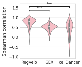
Violinplot#
dfs = []

g_df = pd.DataFrame({"Spearman correlation": cor_cd})
g_df["Method"] = "cellDancer"
dfs.append(g_df)

g_df = pd.DataFrame({"Spearman correlation": cor_rgv})
g_df["Method"] = "RegVelo"
dfs.append(g_df)

g_df = pd.DataFrame({"Spearman correlation": cor_gex})
g_df["Method"] = "GEX"
dfs.append(g_df)

df = pd.concat(dfs, axis=0)
df["Method"] = df["Method"].astype("category")
with mplscience.style_context():
    sns.set_style(style="whitegrid")
    fig, ax = plt.subplots(figsize=(3, 3))
    # pal = {"RegVelo": "#0173b2", "veloVI": "#de8f05"}

    sns.violinplot(
        data=df,
        ax=ax,
        # orient="h",
        x="Method",
        y="Spearman correlation",
        order=["RegVelo", "GEX", "cellDancer"],
        color="lightpink",
    )

    ttest_res = ttest_ind(
        cor_rgv,
        cor_gex,
        equal_var=False,
        alternative="greater",
    )
    significance = get_significance(pvalue=ttest_res.pvalue)
    add_significance(
        ax=ax,
        left=0,
        right=1,
        significance=significance,
        lw=1,
        bracket_level=1.05,
        c="k",
        level=0,
    )

    ttest_res = ttest_ind(
        cor_rgv,
        cor_cd,
        equal_var=False,
        alternative="greater",
    )
    significance = get_significance(pvalue=ttest_res.pvalue)
    add_significance(
        ax=ax,
        left=0,
        right=2,
        significance=significance,
        lw=1,
        bracket_level=1.05,
        c="k",
        level=0,
    )

    plt.xlabel("")

    if SAVE_FIGURES:
        fig.savefig(FIG_DIR / DATASET / "corr_sp.svg", format="svg", transparent=True, bbox_inches="tight")
    plt.show()